目的
単純なしきい値処理
ここでは話は単純である。すべてのピクセルに対して同じしきい値が適用される。ピクセル値がしきい値以下であれば0に設定され、そうでなければ最大値に設定される。しきい値処理を適用するには関数 cv.threshold を使う。第1引数は元画像で、グレースケール画像でなければならない。第2引数はピクセル値を分類するために使うしきい値である。第3引数はしきい値を超えるピクセル値に割り当てられる最大値である。OpenCVはさまざまな種類のしきい値処理を提供しており、これは関数の第4引数で指定する。上記のような基本的なしきい値処理は型 cv.THRESH_BINARY を使って行う。すべての単純なしきい値処理の種類は次のとおりである。
それぞれの違いについては各型のドキュメントを参照のこと。
このメソッドは2つの出力を返す。1つ目は使用されたしきい値で、2つ目の出力はしきい値処理された画像である。
このコードは異なる単純なしきい値処理の種類を比較する。
import cv2 as cv
import numpy as np
from matplotlib import pyplot as plt
img =
cv.imread(
'gradient.png', cv.IMREAD_GRAYSCALE)
assert img is not None, "file could not be read, check with os.path.exists()"
ret,thresh2 =
cv.threshold(img,127,255,cv.THRESH_BINARY_INV)
ret,thresh5 =
cv.threshold(img,127,255,cv.THRESH_TOZERO_INV)
titles = ['Original Image','BINARY','BINARY_INV','TRUNC','TOZERO','TOZERO_INV']
images = [img, thresh1, thresh2, thresh3, thresh4, thresh5]
for i in range(6):
plt.subplot(2,3,i+1),plt.imshow(images[i],'gray',vmin=0,vmax=255)
plt.title(titles[i])
plt.xticks([]),plt.yticks([])
plt.show()
Mat imread(const String &filename, int flags=IMREAD_COLOR_BGR)
Loads an image from a file.
double threshold(InputArray src, OutputArray dst, double thresh, double maxval, int type)
Applies a fixed-level threshold to each array element.
- 覚え書き
- 複数の画像をプロットするために、plt.subplot() 関数を使った。詳細は matplotlib のドキュメントを参照のこと。
このコードは次の結果を生成する。
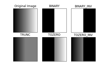
image
適応的しきい値処理
前節では、1つのグローバルな値をしきい値として使った。しかしこれはすべての場合に適しているとは限らない。例えば、画像内の領域ごとに照明条件が異なる場合などである。そのような場合には、適応的しきい値処理が役立つ。ここでは、アルゴリズムが各ピクセルの周囲の小さな領域に基づいてそのピクセルのしきい値を決定する。そのため、同じ画像でも領域ごとに異なるしきい値が得られ、照明にばらつきのある画像に対してより良い結果が得られる。
上で述べた引数に加えて、メソッド cv.adaptiveThreshold は3つの入力引数を取る。
adaptiveMethod はしきい値の計算方法を決定する。
blockSize は近傍領域のサイズを決定し、C は近傍ピクセルの平均または加重和から引かれる定数である。
以下のコードは、照明にばらつきのある画像に対してグローバルしきい値処理と適応的しきい値処理を比較する。
import cv2 as cv
import numpy as np
from matplotlib import pyplot as plt
img =
cv.imread(
'sudoku.png', cv.IMREAD_GRAYSCALE)
assert img is not None, "file could not be read, check with os.path.exists()"
cv.THRESH_BINARY,11,2)
cv.THRESH_BINARY,11,2)
titles = ['Original Image', 'Global Thresholding (v = 127)',
'Adaptive Mean Thresholding', 'Adaptive Gaussian Thresholding']
images = [img, th1, th2, th3]
for i in range(4):
plt.subplot(2,2,i+1),plt.imshow(images[i],'gray')
plt.title(titles[i])
plt.xticks([]),plt.yticks([])
plt.show()
void medianBlur(InputArray src, OutputArray dst, int ksize)
Blurs an image using the median filter.
void adaptiveThreshold(InputArray src, OutputArray dst, double maxValue, int adaptiveMethod, int thresholdType, int blockSize, double C)
Applies an adaptive threshold to an array.
結果:
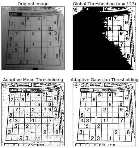
image
大津の二値化
グローバルしきい値処理では、任意に選んだ値をしきい値として使った。これに対して、大津の手法では値を選ぶ必要がなく、自動的に決定する。
2つの異なる画像値のみを持つ画像(バイモーダル画像)を考えると、ヒストグラムは2つのピークだけで構成される。良いしきい値はこれら2つの値の中間にあるだろう。同様に、大津の手法は画像のヒストグラムから最適なグローバルしきい値を決定する。
そのために cv.threshold() 関数を使い、追加のフラグとして cv.THRESH_OTSU を渡す。しきい値は任意に選んでよい。するとアルゴリズムが最適なしきい値を見つけ、それが1つ目の出力として返される。
以下の例を見てほしい。入力画像はノイズのある画像である。1つ目のケースでは、値127でグローバルしきい値処理を適用する。2つ目のケースでは、大津のしきい値処理を直接適用する。3つ目のケースでは、まず画像を5x5のガウシアンカーネルでフィルタリングしてノイズを除去し、その後に大津のしきい値処理を適用する。ノイズフィルタリングが結果をどのように改善するかを見てほしい。
import cv2 as cv
import numpy as np
from matplotlib import pyplot as plt
img =
cv.imread(
'noisy2.png', cv.IMREAD_GRAYSCALE)
assert img is not None, "file could not be read, check with os.path.exists()"
ret2,th2 =
cv.threshold(img,0,255,cv.THRESH_BINARY+cv.THRESH_OTSU)
ret3,th3 =
cv.threshold(blur,0,255,cv.THRESH_BINARY+cv.THRESH_OTSU)
images = [img, 0, th1,
img, 0, th2,
blur, 0, th3]
titles = ['Original Noisy Image','Histogram','Global Thresholding (v=127)',
'Original Noisy Image','Histogram',"Otsu's Thresholding",
'Gaussian filtered Image','Histogram',"Otsu's Thresholding"]
for i in range(3):
plt.subplot(3,3,i*3+1),plt.imshow(images[i*3],'gray')
plt.title(titles[i*3]), plt.xticks([]), plt.yticks([])
plt.subplot(3,3,i*3+2),plt.hist(images[i*3].ravel(),256)
plt.title(titles[i*3+1]), plt.xticks([]), plt.yticks([])
plt.subplot(3,3,i*3+3),plt.imshow(images[i*3+2],'gray')
plt.title(titles[i*3+2]), plt.xticks([]), plt.yticks([])
plt.show()
void GaussianBlur(InputArray src, OutputArray dst, Size ksize, double sigmaX, double sigmaY=0, int borderType=BORDER_DEFAULT, AlgorithmHint hint=cv::ALGO_HINT_DEFAULT)
Blurs an image using a Gaussian filter.
結果:
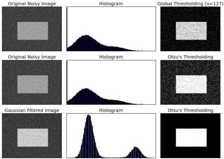
image
大津の二値化はどのように動作するのか?
この節では、大津の二値化が実際にどのように動作するかを示すため、Pythonによる実装を紹介する。興味がなければ読み飛ばしてよい。
バイモーダル画像を扱っているので、大津のアルゴリズムは次の関係式で与えられるクラス内分散の加重和を最小化するしきい値 (t) を見つけようとする。
\[\sigma_w^2(t) = q_1(t)\sigma_1^2(t)+q_2(t)\sigma_2^2(t)\]
ここで
\[q_1(t) = \sum_{i=1}^{t} P(i) \quad \& \quad q_2(t) = \sum_{i=t+1}^{I} P(i)\]
\[\mu_1(t) = \sum_{i=1}^{t} \frac{iP(i)}{q_1(t)} \quad \& \quad \mu_2(t) = \sum_{i=t+1}^{I} \frac{iP(i)}{q_2(t)}\]
\[\sigma_1^2(t) = \sum_{i=1}^{t} [i-\mu_1(t)]^2 \frac{P(i)}{q_1(t)} \quad \& \quad \sigma_2^2(t) = \sum_{i=t+1}^{I} [i-\mu_2(t)]^2 \frac{P(i)}{q_2(t)}\]
実際には、両方のクラスに対する分散が最小になるように、2つのピークの間にある t の値を見つける。これはPythonで次のように簡単に実装できる。
img =
cv.imread(
'noisy2.png', cv.IMREAD_GRAYSCALE)
assert img is not None, "file could not be read, check with os.path.exists()"
hist_norm = hist.ravel()/hist.sum()
Q = hist_norm.cumsum()
bins = np.arange(256)
fn_min = np.inf
thresh = -1
for i in range(1,256):
p1,p2 = np.hsplit(hist_norm,[i])
q1,q2 = Q[i],Q[255]-Q[i]
if q1 < 1.e-6 or q2 < 1.e-6:
continue
b1,b2 = np.hsplit(bins,[i])
m1,m2 = np.sum(p1*b1)/q1, np.sum(p2*b2)/q2
v1,v2 = np.sum(((b1-m1)**2)*p1)/q1,np.sum(((b2-m2)**2)*p2)/q2
fn = v1*q1 + v2*q2
if fn < fn_min:
fn_min = fn
thresh = i
ret, otsu =
cv.threshold(blur,0,255,cv.THRESH_BINARY+cv.THRESH_OTSU)
print( "{} {}".format(thresh,ret) )
void calcHist(const Mat *images, int nimages, const int *channels, InputArray mask, OutputArray hist, int dims, const int *histSize, const float **ranges, bool uniform=true, bool accumulate=false)
Calculates a histogram of a set of arrays.
追加資料
- Digital Image Processing, Rafael C. Gonzalez
演習
- 大津の二値化にはいくつかの最適化が可能である。それを探して実装してみるとよい。