はじめに

このチュートリアルでは、いくつかのコードを用いてホモグラフィの基本的な概念を示す。理論の詳細な説明については、コンピュータビジョンの講義やコンピュータビジョンの書籍を参照してほしい。例えば次のとおり:

Multiple View Geometry in Computer Vision, Richard Hartley and Andrew Zisserman, [121] (一部のサンプル章はこちらで入手可能。CVPRチュートリアルはこちらで入手可能)
An Invitation to 3-D Vision: From Images to Geometric Models, Yi Ma, Stefano Soatto, Jana Kosecka, and S. Shankar Sastry, [184] (コンピュータビジョンの教材はこちらで入手可能)
Computer Vision: Algorithms and Applications, Richard Szeliski, [269] (電子版はこちらで入手可能)
Deeper understanding of the homography decomposition for vision-based control, Ezio Malis, Manuel Vargas, [187] (オープンアクセスはこちら)
Pose Estimation for Augmented Reality: A Hands-On Survey, Eric Marchand, Hideaki Uchiyama, Fabien Spindler, [189] (オープンアクセスはこちら)

チュートリアルコードはこちらにある。C++, Python, Java。このチュートリアルで使用する画像はこちら (left*.jpg) にある。

基本理論

ホモグラフィ行列とは何か?

簡単に言えば、平面ホモグラフィは2つの平面間の変換を(スケール係数を除いて)関係づける。

\[ s \begin{bmatrix} x^{'} \\ y^{'} \\ 1 \end{bmatrix} = \mathbf{H} \begin{bmatrix} x \\ y \\ 1 \end{bmatrix} = \begin{bmatrix} h_{11} & h_{12} & h_{13} \\ h_{21} & h_{22} & h_{23} \\ h_{31} & h_{32} & h_{33} \end{bmatrix} \begin{bmatrix} x \\ y \\ 1 \end{bmatrix} \]

ホモグラフィ行列は 3x3 の行列だが、スケールを除いて推定されるため自由度(DoF)は 8 である。一般に \( h_{33} = 1 \) または \( h_{11}^2 + h_{12}^2 + h_{13}^2 + h_{21}^2 + h_{22}^2 + h_{23}^2 + h_{31}^2 + h_{32}^2 + h_{33}^2 = 1 \) で正規化される(1 も参照)。

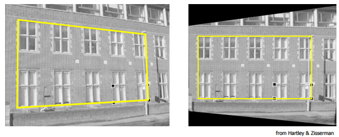
以下の例はさまざまな種類の変換を示しているが、いずれも2つの平面間の変換を関係づけている。

平面と画像平面(画像は 2 より引用)

2つのカメラ位置から見た平面（画像は 3 および 2 より引用）

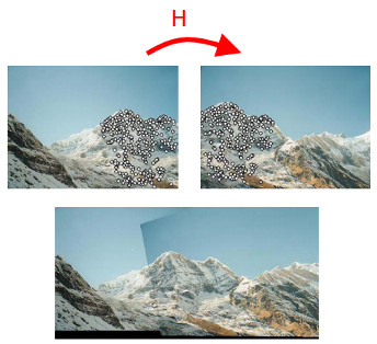
投影軸を中心に回転するカメラ。これは点が無限遠の平面上にあると考えることと等価である（画像は 2 より引用）

ホモグラフィ変換はどのように役立つのか？

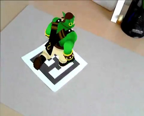
例えばマーカーを使った拡張現実向けの、同一平面上の点からのカメラ姿勢推定（前述の1つ目の例を参照）

透視の除去・補正（前述の2つ目の例を参照）

パノラマのスティッチング（前述の2つ目および3つ目の例を参照）

デモコード

デモ1: 同一平面上の点からの姿勢推定

覚え書き: ホモグラフィからカメラ姿勢を推定するコードはあくまで一例であり、平面物体または任意の物体についてカメラ姿勢を推定したい場合は、代わりにcv::solvePnPを使うべきである。

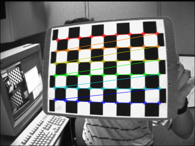
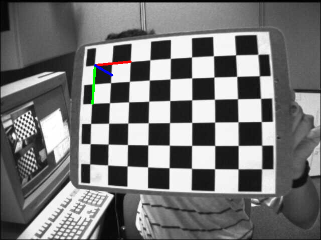
ホモグラフィは、例えば Direct Linear Transform (DLT) アルゴリズムを用いて推定できる（詳細は 1 を参照）。物体が平面であるため、物体フレームで表現された点と、正規化カメラフレームで表現された画像平面への投影点との間の変換はホモグラフィになる。物体が平面である場合に限り、カメラの内部パラメータが既知であればホモグラフィからカメラ姿勢を復元できる（2 または 4 を参照）。これはチェスボードの物体と findChessboardCorners() を用いて画像内のコーナー位置を取得することで、簡単に試すことができる。

まず最初に、チェスボードのコーナーを検出する必要がある。チェスボードのサイズ（patternSize）、ここでは 9x6 が必要となる:

vector<Point2f> corners;

bool found = findChessboardCorners(img, patternSize, corners);

物体フレームで表現された物体点は、チェスボードの正方形のサイズが分かっていれば簡単に計算できる:

 for( int i = 0; i < boardSize.height; i++ )
 for( int j = 0; j < boardSize.width; j++ )
                corners.push_back(Point3f(float(j*squareSize),
 float(i*squareSize), 0));

ホモグラフィ推定の部分では、座標 Z=0 を除去する必要がある:

    vector<Point3f> objectPoints;
    calcChessboardCorners(patternSize, squareSize, objectPoints);
    vector<Point2f> objectPointsPlanar;
 for (size_t i = 0; i < objectPoints.size(); i++)
    {
        objectPointsPlanar.push_back(Point2f(objectPoints[i].x, objectPoints[i].y));
    }

正規化カメラで表現された画像点は、コーナー点から、カメラの内部パラメータと歪み係数を用いて逆透視変換を適用することで計算できる:

 FileStorage fs( samples::findFile( intrinsicsPath ), FileStorage::READ);
 Mat cameraMatrix, distCoeffs;
    fs["camera_matrix"] >> cameraMatrix;
    fs["distortion_coefficients"] >> distCoeffs;

vector<Point2f> imagePoints;

undistortPoints(corners, imagePoints, cameraMatrix, distCoeffs);

ホモグラフィは次のようにして推定できる:

Mat H = findHomography(objectPointsPlanar, imagePoints);

cout << "H:\n" << H << endl;

ホモグラフィ行列から姿勢を求める手早い方法は次のとおりである（5 を参照）:

 // Normalization to ensure that ||c1|| = 1
 double norm = sqrt(H.at<double>(0,0)*H.at<double>(0,0) +
                       H.at<double>(1,0)*H.at<double>(1,0) +
                       H.at<double>(2,0)*H.at<double>(2,0));
 
    H /= norm;
 Mat c1  = H.col(0);
 Mat c2  = H.col(1);
 Mat c3 = c1.cross(c2);
 
 Mat tvec = H.col(2);
 Mat R(3, 3, CV_64F);
 
 for (int i = 0; i < 3; i++)
    {
        R.at<double>(i,0) = c1.at<double>(i,0);
        R.at<double>(i,1) = c2.at<double>(i,0);
        R.at<double>(i,2) = c3.at<double>(i,0);
    }

\[ \begin{align*} \mathbf{X} &= \left( X, Y, 0, 1 \right ) \\ \mathbf{x} &= \mathbf{P}\mathbf{X} \\ &= \mathbf{K} \left[ \mathbf{r_1} \hspace{0.5em} \mathbf{r_2} \hspace{0.5em} \mathbf{r_3} \hspace{0.5em} \mathbf{t} \right ] \begin{pmatrix} X \\ Y \\ 0 \\ 1 \end{pmatrix} \\ &= \mathbf{K} \left[ \mathbf{r_1} \hspace{0.5em} \mathbf{r_2} \hspace{0.5em} \mathbf{t} \right ] \begin{pmatrix} X \\ Y \\ 1 \end{pmatrix} \\ &= \mathbf{H} \begin{pmatrix} X \\ Y \\ 1 \end{pmatrix} \end{align*} \]

\[ \begin{align*} \mathbf{H} &= \lambda \mathbf{K} \left[ \mathbf{r_1} \hspace{0.5em} \mathbf{r_2} \hspace{0.5em} \mathbf{t} \right ] \\ \mathbf{K}^{-1} \mathbf{H} &= \lambda \left[ \mathbf{r_1} \hspace{0.5em} \mathbf{r_2} \hspace{0.5em} \mathbf{t} \right ] \\ \mathbf{P} &= \mathbf{K} \left[ \mathbf{r_1} \hspace{0.5em} \mathbf{r_2} \hspace{0.5em} \left( \mathbf{r_1} \times \mathbf{r_2} \right ) \hspace{0.5em} \mathbf{t} \right ] \end{align*} \]

これは手早い解法である（2 も参照）。この方法では、得られる回転行列が直交することは保証されず、スケールは最初の列を1に正規化することで大まかに推定される。

適切な回転行列（回転行列の性質を満たすもの）を得る解法として、極分解、すなわち回転行列の直交化を適用する方法がある（情報については 6、7、8、または 9 を参照）:

    cout << "R (before polar decomposition):\n" << R << "\ndet(R): " << determinant(R) << endl;
 Mat_<double> W, U, Vt;
 SVDecomp(R, W, U, Vt);
    R = U*Vt;
 double det = determinant(R);
 if (det < 0)
    {
        Vt.at<double>(2,0) *= -1;
        Vt.at<double>(2,1) *= -1;
        Vt.at<double>(2,2) *= -1;
 
        R = U*Vt;
    }
    cout << "R (after polar decomposition):\n" << R << "\ndet(R): " << determinant(R) << endl;

結果を確認するため、推定したカメラ姿勢を用いて画像に投影した物体フレームを表示する:

デモ2: 透視補正

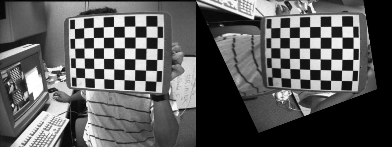
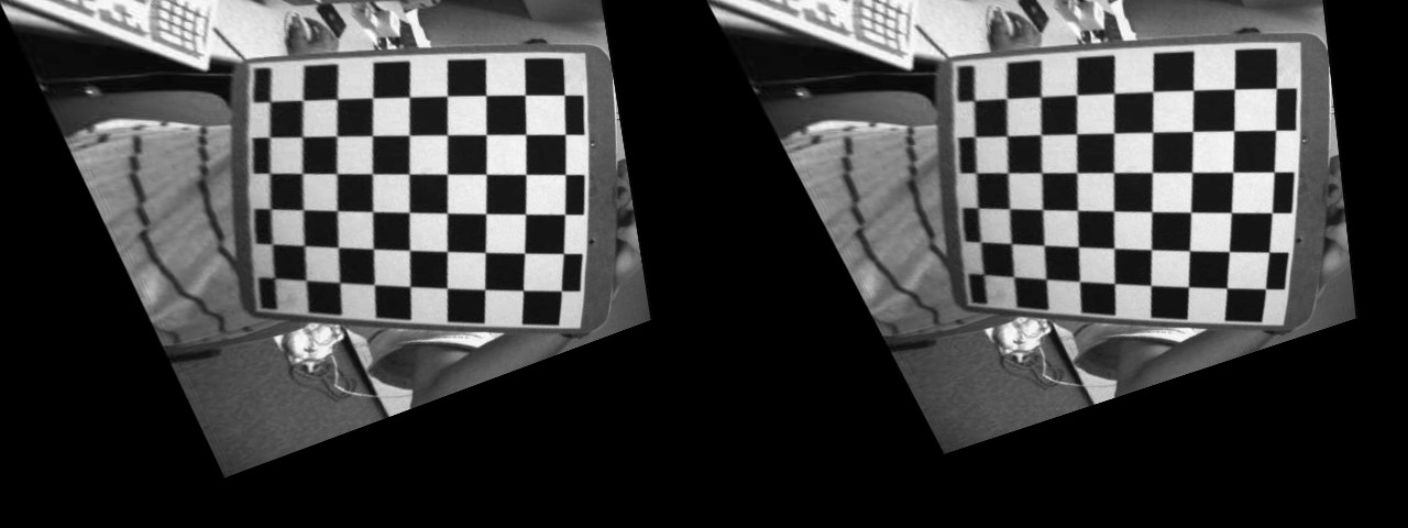
この例では、ソース点を目的の点に対応付けるホモグラフィを計算することで、ソース画像を望みの透視ビューに変換する。次の画像は、ソース画像（左）と、望みのチェスボードビューへ変換したいチェスボードビュー（右）を示している。

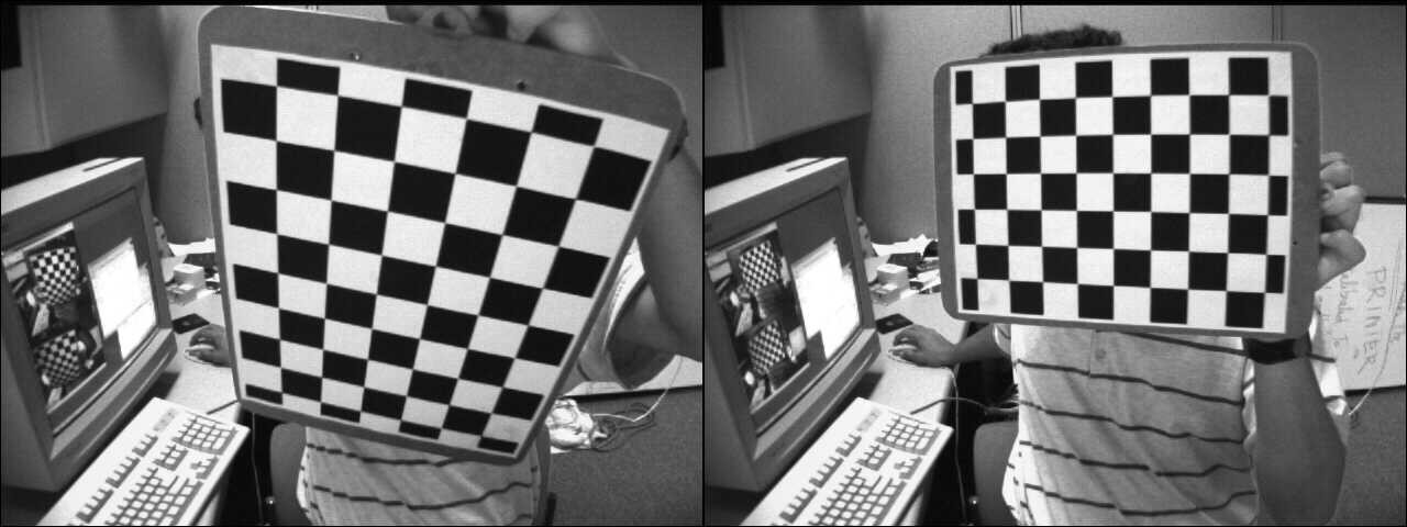
Source and desired views

最初のステップとして、ソース画像と目的画像でチェスボードのコーナーを検出する:

ホモグラフィは次のように簡単に推定できる:

元のチェスボード視点を目的のチェスボード視点へワープするために、cv::warpPerspectiveを使用する。

結果画像は次のとおりである:

ホモグラフィによって変換されたソースコーナーの座標を計算するには:

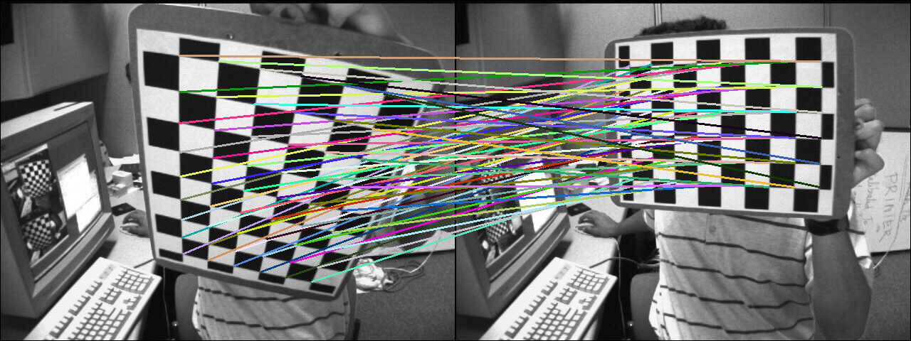
計算の正しさを確認するため、対応する線分を表示する:

デモ3: カメラの変位からのホモグラフィ

ホモグラフィは2つの平面間の変換を関係づけており、最初の平面視点から2番目の平面視点へ移動できる対応するカメラ変位を取り出すことが可能である(詳細は[187]を参照)。カメラ変位からホモグラフィを計算する詳細に入る前に、カメラ姿勢と同次変換についていくつか復習しておく。

関数cv::solvePnPは、3D物体点(物体フレームで表された点)とそれを投影した2D画像点(画像内で見える物体点)との対応からカメラ姿勢を計算できる。内部パラメータと歪み係数が必要である(カメラキャリブレーション処理を参照)。

\[ \begin{align*} s \begin{bmatrix} u \\ v \\ 1 \end{bmatrix} &= \begin{bmatrix} f_x & 0 & c_x \\ 0 & f_y & c_y \\ 0 & 0 & 1 \end{bmatrix} \begin{bmatrix} r_{11} & r_{12} & r_{13} & t_x \\ r_{21} & r_{22} & r_{23} & t_y \\ r_{31} & r_{32} & r_{33} & t_z \end{bmatrix} \begin{bmatrix} X_o \\ Y_o \\ Z_o \\ 1 \end{bmatrix} \\ &= \mathbf{K} \hspace{0.2em} ^{c}\mathbf{M}_o \begin{bmatrix} X_o \\ Y_o \\ Z_o \\ 1 \end{bmatrix} \end{align*} \]

\( \mathbf{K} \) は内部パラメータ行列、\( ^{c}\mathbf{M}_o \) はカメラ姿勢である。cv::solvePnPの出力はまさにこれであり、rvecはロドリゲス回転ベクトル、tvecは並進ベクトルである。

\( ^{c}\mathbf{M}_o \) は同次形式で表現でき、物体フレームで表現された点をカメラフレームへ変換できる:

\[ \begin{align*} \begin{bmatrix} X_c \\ Y_c \\ Z_c \\ 1 \end{bmatrix} &= \hspace{0.2em} ^{c}\mathbf{M}_o \begin{bmatrix} X_o \\ Y_o \\ Z_o \\ 1 \end{bmatrix} \\ &= \begin{bmatrix} ^{c}\mathbf{R}_o & ^{c}\mathbf{t}_o \\ 0_{1\times3} & 1 \end{bmatrix} \begin{bmatrix} X_o \\ Y_o \\ Z_o \\ 1 \end{bmatrix} \\ &= \begin{bmatrix} r_{11} & r_{12} & r_{13} & t_x \\ r_{21} & r_{22} & r_{23} & t_y \\ r_{31} & r_{32} & r_{33} & t_z \\ 0 & 0 & 0 & 1 \end{bmatrix} \begin{bmatrix} X_o \\ Y_o \\ Z_o \\ 1 \end{bmatrix} \end{align*} \]

あるフレームで表現された点を別のフレームへ変換することは、行列の乗算で簡単に行える:

\( ^{c_1}\mathbf{M}_o \) はカメラ1のカメラ姿勢である
\( ^{c_2}\mathbf{M}_o \) はカメラ2のカメラ姿勢である

カメラ1フレームで表現された3D点をカメラ2フレームへ変換するには:

\[ ^{c_2}\mathbf{M}_{c_1} = \hspace{0.2em} ^{c_2}\mathbf{M}_{o} \cdot \hspace{0.1em} ^{o}\mathbf{M}_{c_1} = \hspace{0.2em} ^{c_2}\mathbf{M}_{o} \cdot \hspace{0.1em} \left( ^{c_1}\mathbf{M}_{o} \right )^{-1} = \begin{bmatrix} ^{c_2}\mathbf{R}_{o} & ^{c_2}\mathbf{t}_{o} \\ 0_{3 \times 1} & 1 \end{bmatrix} \cdot \begin{bmatrix} ^{c_1}\mathbf{R}_{o}^T & - \hspace{0.2em} ^{c_1}\mathbf{R}_{o}^T \cdot \hspace{0.2em} ^{c_1}\mathbf{t}_{o} \\ 0_{1 \times 3} & 1 \end{bmatrix} \]

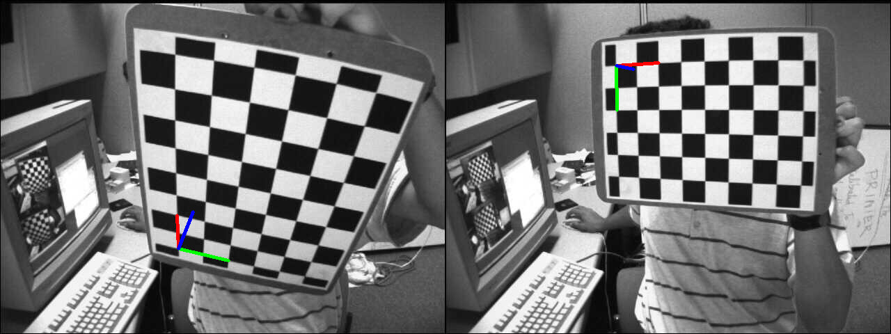
この例では、チェスボードの物体を基準として、2つのカメラ姿勢間のカメラの変位を計算する。最初のステップとして、2枚の画像についてカメラ姿勢を計算する:

    vector<Point2f> corners1, corners2;
 bool found1 = findChessboardCorners(img1, patternSize, corners1);
 bool found2 = findChessboardCorners(img2, patternSize, corners2);
 
 if (!found1 || !found2)
    {
        cout << "Error, cannot find the chessboard corners in both images." << endl;
 return;
    }
 
    vector<Point3f> objectPoints;
    calcChessboardCorners(patternSize, squareSize, objectPoints);
 
 FileStorage fs( samples::findFile( intrinsicsPath ), FileStorage::READ);
 Mat cameraMatrix, distCoeffs;
    fs["camera_matrix"] >> cameraMatrix;
    fs["distortion_coefficients"] >> distCoeffs;
 
 Mat rvec1, tvec1;
 solvePnP(objectPoints, corners1, cameraMatrix, distCoeffs, rvec1, tvec1);
 Mat rvec2, tvec2;
 solvePnP(objectPoints, corners2, cameraMatrix, distCoeffs, rvec2, tvec2);

カメラの変位は、上記の式を用いてカメラ姿勢から計算できる:

void computeC2MC1(const Mat &R1, const Mat &tvec1, const Mat &R2, const Mat &tvec2,
 Mat &R_1to2, Mat &tvec_1to2)
{
 //c2Mc1 = c2Mo * oMc1 = c2Mo * c1Mo.inv()
    R_1to2 = R2 * R1.t();
    tvec_1to2 = R2 * (-R1.t()*tvec1) + tvec2;
}

カメラの変位から計算される、特定の平面に関連するホモグラフィは次のとおりである:

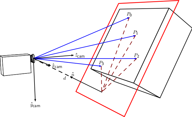
By Homography-transl.svg: Per Rosengren derivative work: Appoose (Homography-transl.svg) [CC BY 3.0 (http://creativecommons.org/licenses/by/3.0)], via Wikimedia Commons

この図において、n は平面の法線ベクトル、d は平面の法線方向に沿ったカメラフレームと平面との距離である。カメラの変位からホモグラフィを計算する式は次のとおりである:

\[ ^{2}\mathbf{H}_{1} = \hspace{0.2em} ^{2}\mathbf{R}_{1} - \hspace{0.1em} \frac{^{2}\mathbf{t}_{1} \cdot \hspace{0.1em} ^{1}\mathbf{n}^\top}{^1d} \]

ここで \( ^{2}\mathbf{H}_{1} \) は、1つ目のカメラフレーム内の点を2つ目のカメラフレーム内の対応する点へ対応付けるホモグラフィ行列であり、\( ^{2}\mathbf{R}_{1} = \hspace{0.2em} ^{c_2}\mathbf{R}_{o} \cdot \hspace{0.1em} ^{c_1}\mathbf{R}_{o}^{\top} \) は2つのカメラフレーム間の回転を表す回転行列、\( ^{2}\mathbf{t}_{1} = \hspace{0.2em} ^{c_2}\mathbf{R}_{o} \cdot \left( - \hspace{0.1em} ^{c_1}\mathbf{R}_{o}^{\top} \cdot \hspace{0.1em} ^{c_1}\mathbf{t}_{o} \right ) + \hspace{0.1em} ^{c_2}\mathbf{t}_{o} \) は2つのカメラフレーム間の並進ベクトルである。

ここで法線ベクトル n はカメラフレーム1で表現された平面の法線であり、（平面上にある同一直線上にない3点を用いて）2つのベクトルの外積として計算できる。あるいは本例では次のように直接計算できる:

Mat normal = Mat_<double>({3,1}, {0, 0, 1});

Mat normal1 = R1*normal;

距離 d は、平面の法線と平面上の点との内積として計算するか、または平面の方程式を計算してD係数を用いることで計算できる:

 Mat origin(3, 1, CV_64F, Scalar(0));
 Mat origin1 = R1*origin + tvec1;
 double d_inv1 = 1.0 / normal1.dot(origin1);

射影ホモグラフィ行列 \( \textbf{G} \) は、内部パラメータ行列 \( \textbf{K} \) を用いてユークリッドホモグラフィ \( \textbf{H} \) から計算できる([187]を参照)。ここでは2つの平面視点で同じカメラを使用していると仮定する。

\[ \textbf{G} = \gamma \textbf{K} \textbf{H} \textbf{K}^{-1} \]

Mat computeHomography(const Mat &R_1to2, const Mat &tvec_1to2, const double d_inv, const Mat &normal)
{
 Mat homography = R_1to2 + d_inv * tvec_1to2*normal.t();
 return homography;
}

本例ではチェスボードのZ軸は物体の内側を向くが、ホモグラフィの図では外側を向く。これは単に符号の問題である:

\[ ^{2}\mathbf{H}_{1} = \hspace{0.2em} ^{2}\mathbf{R}_{1} + \hspace{0.1em} \frac{^{2}\mathbf{t}_{1} \cdot \hspace{0.1em} ^{1}\mathbf{n}^\top}{^1d} \]

 Mat homography_euclidean = computeHomography(R_1to2, t_1to2, d_inv1, normal1);
 Mat homography = cameraMatrix * homography_euclidean * cameraMatrix.inv();
 
    homography /= homography.at<double>(2,2);
    homography_euclidean /= homography_euclidean.at<double>(2,2);

ここで、カメラ変位から計算した射影ホモグラフィと、cv::findHomographyで推定したものとを比較する。

findHomography H:
[0.32903393332201, -1.244138808862929, 536.4769088231476;
 0.6969763913334046, -0.08935909072571542, -80.34068504082403;
 0.00040511729592961, -0.001079740100565013, 0.9999999999999999]
 
homography from camera displacement:
[0.4160569997384721, -1.306889006892538, 553.7055461075881;
 0.7917584252773352, -0.06341244158456338, -108.2770029401219;
 0.0005926357240956578, -0.001020651672127799, 1]

ホモグラフィ行列は類似している。両方のホモグラフィ行列を用いてワープした画像1を比較すると:

Left: image warped using the estimated homography. Right: using the homography computed from the camera displacement.

視覚的には、カメラ変位から計算したホモグラフィによる結果画像と、cv::findHomography関数で推定したものとの違いを見分けるのは難しい。

演習

このデモでは、2つのカメラ姿勢からホモグラフィ変換を計算する方法を示している。今度は、N個の中間ホモグラフィを計算して同じ操作を行ってみてほしい。1つのホモグラフィを計算してソース画像を望みのカメラ視点へ直接ワープする代わりに、N回のワープ操作を行い、それぞれの変換が働く様子を確認する。

次のような結果が得られるはずである:

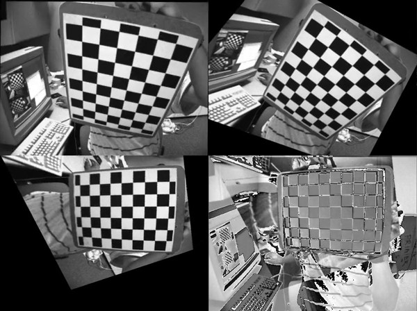
The first three images show the source image warped at three different interpolated camera viewpoints. The 4th image shows the "error image" between the warped source image at the final camera viewpoint and the desired image.

デモ4: ホモグラフィ行列の分解

OpenCV 3には関数cv::decomposeHomographyMatが含まれており、ホモグラフィ行列を回転・並進・平面法線の集合に分解できる。まず、カメラ変位から計算したホモグラフィ行列を分解する。

 Mat homography_euclidean = computeHomography(R_1to2, t_1to2, d_inv1, normal1);
 Mat homography = cameraMatrix * homography_euclidean * cameraMatrix.inv();
 
    homography /= homography.at<double>(2,2);
    homography_euclidean /= homography_euclidean.at<double>(2,2);

cv::decomposeHomographyMatの結果は次のとおりである。

    vector<Mat> Rs_decomp, ts_decomp, normals_decomp;
 int solutions = decomposeHomographyMat(homography, cameraMatrix, Rs_decomp, ts_decomp, normals_decomp);
    cout << "Decompose homography matrix computed from the camera displacement:" << endl << endl;
 for (int i = 0; i < solutions; i++)
    {
 double factor_d1 = 1.0 / d_inv1;
 Mat rvec_decomp;
 Rodrigues(Rs_decomp[i], rvec_decomp);
      cout << "Solution " << i << ":" << endl;
      cout << "rvec from homography decomposition: " << rvec_decomp.t() << endl;
      cout << "rvec from camera displacement: " << rvec_1to2.t() << endl;
      cout << "tvec from homography decomposition: " << ts_decomp[i].t() << " and scaled by d: " << factor_d1 * ts_decomp[i].t() << endl;
      cout << "tvec from camera displacement: " << t_1to2.t() << endl;
      cout << "plane normal from homography decomposition: " << normals_decomp[i].t() << endl;
      cout << "plane normal at camera 1 pose: " << normal1.t() << endl << endl;
    }

Solution 0:
rvec from homography decomposition: [-0.0919829920641369, -0.5372581036567992, 1.310868863540717]
rvec from camera displacement: [-0.09198299206413783, -0.5372581036567995, 1.310868863540717]
tvec from homography decomposition: [-0.7747961019053186, -0.02751124463434032, -0.6791980037590677] and scaled by d: [-0.1578091561210742, -0.005603443652993778, -0.1383378976078466]
tvec from camera displacement: [0.1578091561210745, 0.005603443652993617, 0.1383378976078466]
plane normal from homography decomposition: [-0.1973513139420648, 0.6283451996579074, -0.7524857267431757]
plane normal at camera 1 pose: [0.1973513139420654, -0.6283451996579068, 0.752485726743176]
 
Solution 1:
rvec from homography decomposition: [-0.0919829920641369, -0.5372581036567992, 1.310868863540717]
rvec from camera displacement: [-0.09198299206413783, -0.5372581036567995, 1.310868863540717]
tvec from homography decomposition: [0.7747961019053186, 0.02751124463434032, 0.6791980037590677] and scaled by d: [0.1578091561210742, 0.005603443652993778, 0.1383378976078466]
tvec from camera displacement: [0.1578091561210745, 0.005603443652993617, 0.1383378976078466]
plane normal from homography decomposition: [0.1973513139420648, -0.6283451996579074, 0.7524857267431757]
plane normal at camera 1 pose: [0.1973513139420654, -0.6283451996579068, 0.752485726743176]
 
Solution 2:
rvec from homography decomposition: [0.1053487907109967, -0.1561929144786397, 1.401356552358475]
rvec from camera displacement: [-0.09198299206413783, -0.5372581036567995, 1.310868863540717]
tvec from homography decomposition: [-0.4666552552894618, 0.1050032934770042, -0.913007654671646] and scaled by d: [-0.0950475510338766, 0.02138689274867372, -0.1859598508065552]
tvec from camera displacement: [0.1578091561210745, 0.005603443652993617, 0.1383378976078466]
plane normal from homography decomposition: [-0.3131715472900788, 0.8421206145721947, -0.4390403768225507]
plane normal at camera 1 pose: [0.1973513139420654, -0.6283451996579068, 0.752485726743176]
 
Solution 3:
rvec from homography decomposition: [0.1053487907109967, -0.1561929144786397, 1.401356552358475]
rvec from camera displacement: [-0.09198299206413783, -0.5372581036567995, 1.310868863540717]
tvec from homography decomposition: [0.4666552552894618, -0.1050032934770042, 0.913007654671646] and scaled by d: [0.0950475510338766, -0.02138689274867372, 0.1859598508065552]
tvec from camera displacement: [0.1578091561210745, 0.005603443652993617, 0.1383378976078466]
plane normal from homography decomposition: [0.3131715472900788, -0.8421206145721947, 0.4390403768225507]
plane normal at camera 1 pose: [0.1973513139420654, -0.6283451996579068, 0.752485726743176]

ホモグラフィ行列の分解結果は、法線が単位長であるため、実際には距離 d に相当するスケール係数の不定性を除いてのみ復元できる。ご覧のとおり、計算したカメラの変位とほぼ完全に一致する解が1つ存在する。ドキュメントに記載されているとおり:

At least two of the solutions may further be invalidated if point correspondences are available by applying positive depth constraint (all points must be in front of the camera).

分解の結果はカメラの変位であるため、初期カメラ姿勢 \( ^{c_1}\mathbf{M}_{o} \) が得られていれば、現在のカメラ姿勢 \( ^{c_2}\mathbf{M}_{o} = \hspace{0.2em} ^{c_2}\mathbf{M}_{c_1} \cdot \hspace{0.1em} ^{c_1}\mathbf{M}_{o} \) を計算でき、平面に属する3D物体点がカメラの前方に投影されるかどうかを検証できる。もう1つの解法として、カメラ1の姿勢で表現された平面の法線が分かっていれば、最も近い法線を持つ解を採用することも考えられる。

cv::findHomographyで推定したホモグラフィ行列でも同じことを行う。

Solution 0:
rvec from homography decomposition: [0.1552207729599141, -0.152132696119647, 1.323678695078694]
rvec from camera displacement: [-0.09198299206413783, -0.5372581036567995, 1.310868863540717]
tvec from homography decomposition: [-0.4482361704818117, 0.02485247635491922, -1.034409687207331] and scaled by d: [-0.09129598307571339, 0.005061910238634657, -0.2106868109173855]
tvec from camera displacement: [0.1578091561210745, 0.005603443652993617, 0.1383378976078466]
plane normal from homography decomposition: [-0.1384902722707529, 0.9063331452766947, -0.3992250922214516]
plane normal at camera 1 pose: [0.1973513139420654, -0.6283451996579068, 0.752485726743176]
 
Solution 1:
rvec from homography decomposition: [0.1552207729599141, -0.152132696119647, 1.323678695078694]
rvec from camera displacement: [-0.09198299206413783, -0.5372581036567995, 1.310868863540717]
tvec from homography decomposition: [0.4482361704818117, -0.02485247635491922, 1.034409687207331] and scaled by d: [0.09129598307571339, -0.005061910238634657, 0.2106868109173855]
tvec from camera displacement: [0.1578091561210745, 0.005603443652993617, 0.1383378976078466]
plane normal from homography decomposition: [0.1384902722707529, -0.9063331452766947, 0.3992250922214516]
plane normal at camera 1 pose: [0.1973513139420654, -0.6283451996579068, 0.752485726743176]
 
Solution 2:
rvec from homography decomposition: [-0.2886605671759886, -0.521049903923871, 1.381242030882511]
rvec from camera displacement: [-0.09198299206413783, -0.5372581036567995, 1.310868863540717]
tvec from homography decomposition: [-0.8705961357284295, 0.1353018038908477, -0.7037702049789747] and scaled by d: [-0.177321544550518, 0.02755804196893467, -0.1433427218822783]
tvec from camera displacement: [0.1578091561210745, 0.005603443652993617, 0.1383378976078466]
plane normal from homography decomposition: [-0.2284582117722427, 0.6009247303964522, -0.7659610393954643]
plane normal at camera 1 pose: [0.1973513139420654, -0.6283451996579068, 0.752485726743176]
 
Solution 3:
rvec from homography decomposition: [-0.2886605671759886, -0.521049903923871, 1.381242030882511]
rvec from camera displacement: [-0.09198299206413783, -0.5372581036567995, 1.310868863540717]
tvec from homography decomposition: [0.8705961357284295, -0.1353018038908477, 0.7037702049789747] and scaled by d: [0.177321544550518, -0.02755804196893467, 0.1433427218822783]
tvec from camera displacement: [0.1578091561210745, 0.005603443652993617, 0.1383378976078466]
plane normal from homography decomposition: [0.2284582117722427, -0.6009247303964522, 0.7659610393954643]
plane normal at camera 1 pose: [0.1973513139420654, -0.6283451996579068, 0.752485726743176]

ここでも、計算したカメラの変位と一致する解が存在する。

デモ5: 回転するカメラからの基本的なパノラマスティッチング

覚え書き: この例は、カメラの純粋な回転運動に基づく画像スティッチングの概念を示すために作られたものであり、パノラマ画像のスティッチングに使用すべきではない。スティッチングモジュールは画像をスティッチングするための完全なパイプラインを提供している。

ホモグラフィ変換は平面構造に対してのみ適用される。しかしカメラが回転する場合（カメラの投影軸を中心とした純粋な回転で並進がない場合）は、任意の世界を考えることができる（前述を参照）。

そしてホモグラフィは、回転変換とカメラの内部パラメータを用いて次のように計算できる（例えば 10 を参照）:

\[ s \begin{bmatrix} x^{'} \\ y^{'} \\ 1 \end{bmatrix} = \bf{K} \hspace{0.1em} \bf{R} \hspace{0.1em} \bf{K}^{-1} \begin{bmatrix} x \\ y \\ 1 \end{bmatrix} \]

説明のために、無料でオープンソースの3Dコンピュータグラフィックスソフトウェアである Blender を使用し、互いに回転変換のみを持つ2つのカメラビューを生成した。カメラの内部パラメータと、世界に対する 3x4 の外部行列を Blender で取得する方法の詳細は 11 に記載されている（カメラフレームと物体フレーム間の変換を得るには追加の変換が必要となる）。

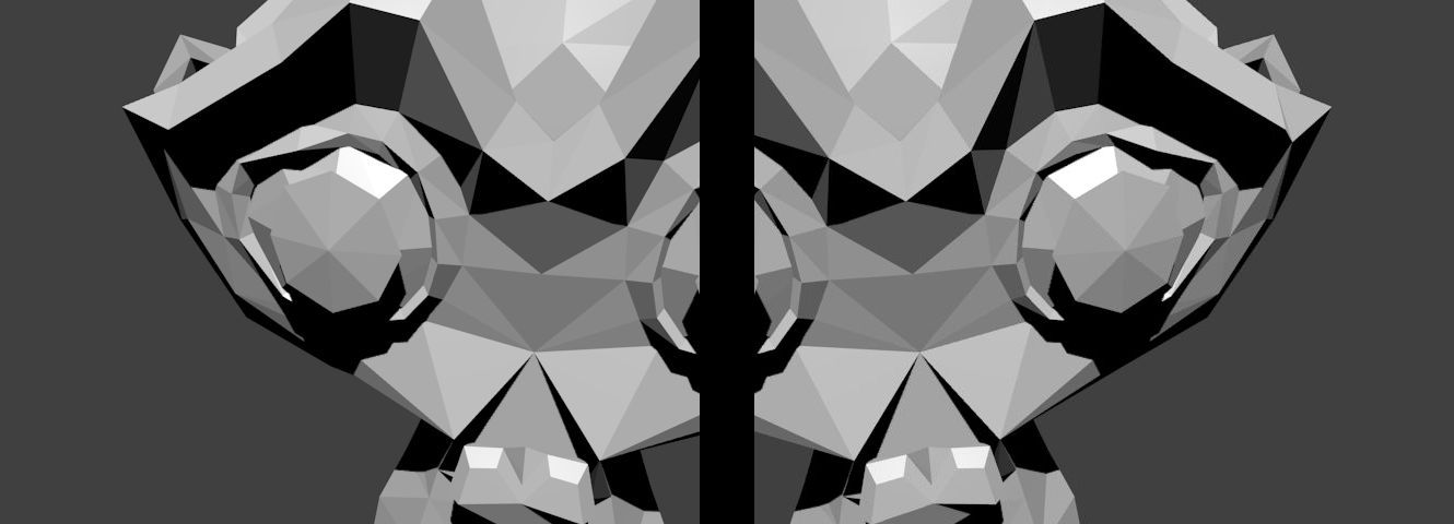
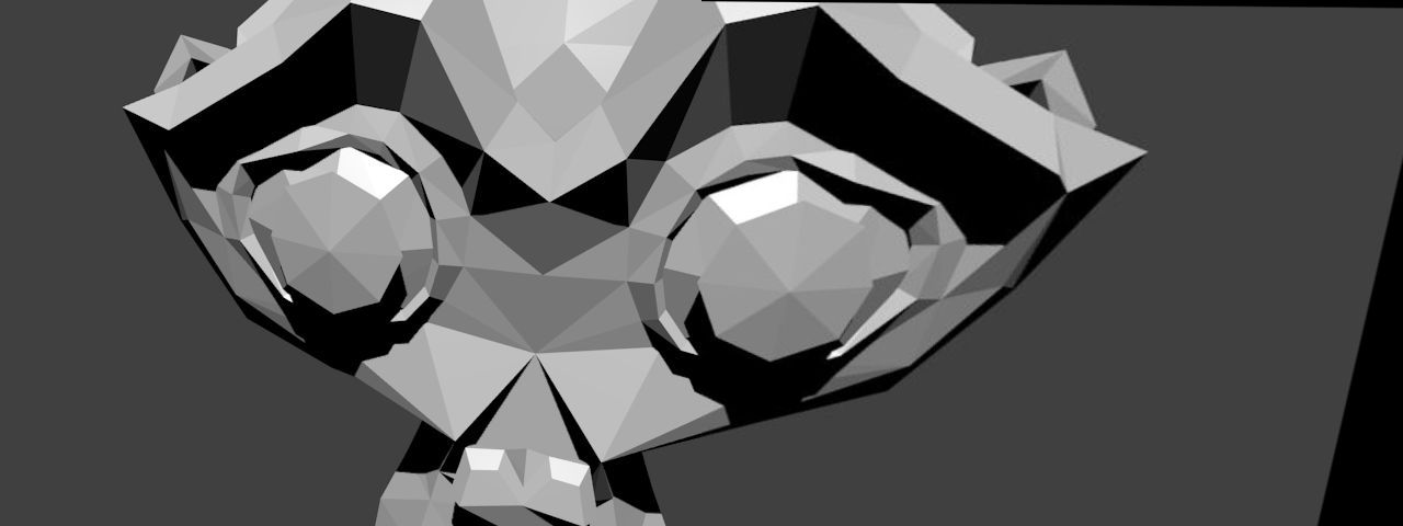
下の図は、回転変換のみを伴って生成された Suzanne モデルの2つのビューを示している:

既知の対応するカメラ姿勢と内部パラメータを用いて、2つのビュー間の相対回転を計算できる:

ここでは、2枚目の画像を1枚目の画像を基準としてスティッチングする。ホモグラフィは上記の式を用いて計算できる:

スティッチングは単純に次のように行う: