|
OpenCV 5.0.0
Open Source Computer Vision
|
読み込み中...
検索中...
見つかりません
|
OpenCV 5.0.0
Open Source Computer Vision
|
OpenCV (Open Source Computer Vision) は、Intel が1999年に開始した人気のコンピュータビジョンライブラリである。このクロスプラットフォームのライブラリはリアルタイムの画像処理に焦点を当てており、最新のコンピュータビジョンアルゴリズムの特許フリーな実装を含む。2008年に Willow Garage がサポートを引き継ぎ、OpenCV 2.3.1 では現在、C、C++、Python、Android へのプログラミングインターフェースが提供されている。OpenCVはBSDライセンスの下でリリースされており、学術プロジェクトでも商用製品でも同様に利用されている。
OpenCV 2.4 では顔認識のための非常に新しいFaceRecognizerクラスが提供されるようになり、すぐに顔認識の実験を始められる。本ドキュメントは、私自身が顔認識に取り組み始めたときに欲しかったガイドである。OpenCVのFaceRecognizerを用いて顔認識を行う方法を(完全なソースコードのリスト付きで)示し、その背後にあるアルゴリズムへの導入を行う。また、多くの論文で見られるような可視化を作成する方法も示す。これは多くの人から要望があったためである。
現在利用可能なアルゴリズムは以下のとおり:
本ページのソースコード例をコピー&ペーストする必要はない。これらは本ドキュメントに付属するsrcフォルダに含まれているからである。サンプルを有効にしてOpenCVをビルドしていれば、すでにコンパイル済みの可能性が高い。非常に上級のユーザーには興味深いかもしれないが、新しいユーザーを混乱させる恐れがあるため、実装の詳細は割愛することにした。
本ドキュメント内のすべてのコードは BSDライセンス の下でリリースされているため、自分のプロジェクトで自由に使用してかまわない。
顔認識は人間にとっては簡単なタスクである。[285] の実験では、生後1〜3日の赤ちゃんでさえも、知っている顔を区別できることが示されている。では、コンピュータにとってはどれほど難しいのだろうか。実は、人間の認識については現在でもほとんど分かっていない。顔認識の成功に使われるのは内側の特徴(目、鼻、口)なのか、それとも外側の特徴(頭の形、生え際)なのか。我々はどのように画像を分析し、脳はそれをどのように符号化しているのか。David Hubel と Torsten Wiesel によって、我々の脳には線、エッジ、角度、動きといったシーンの特定の局所的特徴に反応する特化した神経細胞があることが示された。我々は世界をばらばらの断片としては見ていないため、視覚野はこれらの異なる情報源を何らかの方法で組み合わせて有用なパターンにしているはずである。自動顔認識とは、画像からそうした意味のある特徴を抽出し、それを有用な表現にまとめ、その上で何らかの分類を行うことに尽きる。
顔の幾何学的特徴に基づく顔認識は、おそらく顔認識に対する最も直感的なアプローチである。最初期の自動顔認識システムの一つが [146] で述べられている:マーカ点(目、耳、鼻などの位置)を用いて特徴ベクトル(点間の距離、点同士のなす角度など)を構築した。認識は、プローブ画像と参照画像の特徴ベクトル間のユークリッド距離を計算することで行われた。このような手法はその性質上、照明の変化に対して頑健であるが、大きな欠点がある:最新のアルゴリズムを用いても、マーカ点の正確な位置合わせは難しい。幾何学的顔認識に関する最新の研究の一部は [45] で行われた。22次元の特徴ベクトルが用いられ、大規模なデータセットでの実験により、幾何学的特徴だけでは顔認識に十分な情報を持っていない可能性があることが示された。
[286] で述べられているEigenfaces法は、顔認識に対して全体論的(holistic)なアプローチを取った:顔画像は高次元の画像空間における1点であり、分類が容易になるような低次元の表現を見つける。低次元の部分空間は、分散が最大となる軸を特定する主成分分析(Principal Component Analysis)によって見つけられる。この種の変換は再構成の観点からは最適であるが、クラスラベルをまったく考慮しない。分散が外部要因、例えば光から生じる状況を想像してほしい。分散が最大となる軸が必ずしも識別に役立つ情報を含んでいるとは限らず、その結果、分類が不可能になる。そこで、線形判別分析(Linear Discriminant Analysis)を用いたクラス固有の射影が [25] で顔認識に適用された。基本的な考え方は、クラス内の分散を最小化すると同時に、クラス間の分散を最大化することである。
最近、局所特徴抽出のためのさまざまな手法が登場した。入力データの高次元性を避けるために、画像の局所領域のみを記述する。抽出された特徴は(うまくいけば)部分的な遮蔽、照明、小さなサンプルサイズに対してより頑健である。局所特徴抽出に使われるアルゴリズムには、ガボールウェーブレット(Gabor Wavelets)([308])、離散コサイン変換(Discrete Cosinus Transform)([196])、Local Binary Patterns([4])などがある。局所特徴抽出を適用する際に空間情報を保持する最良の方法は何かは、いまだに未解決の研究課題である。空間情報は潜在的に有用な情報だからである。
まず実験するためのデータを用意しよう。ここではおもちゃのような例を扱いたくはない。顔認識を行うので、いくつかの顔画像が必要になる。独自のデータセットを作成してもよいし、利用可能な顔データベースの一つから始めてもよい。http://face-rec.org/databases/ に最新の概要がある。興味深いデータベースを3つ挙げる(説明の一部は http://face-rec.org から引用している):
Yale Facedatabase A、Yalefacesとしても知られる。AT&T Facedatabaseは初期テストには適しているが、かなり簡単なデータベースである。Eigenfaces法はすでにこのデータベースで97%の認識率を達成しているため、他のアルゴリズムでも大きな改善は見られないだろう。Yale Facedatabase A(Yalefacesとしても知られる)は、認識問題がより難しいため、初期実験により適したデータセットである。このデータベースは15人(男性14人、女性1人)から構成され、それぞれが \(320 \times 243\) ピクセルのグレースケール画像を11枚ずつ持つ。光の条件(中央光、左光、右光)、表情(幸せ、普通、悲しい、眠そう、驚き、ウインク)、眼鏡(眼鏡あり、眼鏡なし)に変化がある。
元の画像はクロップや位置合わせがされていない。その作業を代行するPythonスクリプトについては 付録 を参照してほしい。
データを取得したら、プログラムでそれを読み込む必要がある。デモアプリケーションでは、非常に単純なCSVファイルから画像を読み込むことにした。なぜか。それは私が思いつく最も単純でプラットフォームに依存しないアプローチだからである。ただし、より単純な解決策をご存じであれば教えてほしい。基本的にCSVファイルに含める必要があるのは、ファイル名に続いて ; が続き、その後にラベル(整数として)が続く行だけで、次のような行を構成する:
この行を分解してみよう。/path/to/image.ext は画像へのパスであり、Windowsを使っているならおそらく C:/faces/person0/image0.jpg のようなものになる。次に区切り文字 ; があり、最後にこの画像にラベル 0 を割り当てる。ラベルはこの画像が属する被験者(人物)と考えればよい。したがって同じ被験者(人物)は同じラベルを持つべきである。
AT&T FacedatabaseをAT&T Facedatabaseからダウンロードし、対応するCSVファイルをat.txtからダウンロードする。これは次のようになる(もちろん実際のファイルには ... は含まれない):
ファイルを D:/data/at に展開し、CSVファイルを D:/data/at.txt にダウンロードしたとする。そうしたら、単に ./ を D:/data/ に検索&置換すればよい。これは好みのエディタで行うことができ、十分に高機能なエディタであればどれでもこれが可能である。有効なファイル名とラベルを持つCSVファイルができたら、CSVファイルへのパスをパラメータとして渡すことで、任意のデモを実行できる:
CSVファイルの作成の詳細については、CSVファイルの作成 を参照してほしい。
与えられた画像表現の問題は、その高次元性にある。2次元の \(p \times q\) グレースケール画像は \(m = pq\) 次元のベクトル空間を張るため、\(100 \times 100\) ピクセルの画像はすでに \(10,000\) 次元の画像空間に存在することになる。問題は、すべての次元が我々にとって等しく有用なのかということである。我々はデータに何らかの分散がある場合にのみ判断を下すことができるので、我々が探しているのは情報の大部分を占める成分である。主成分分析(PCA)は、Karl Pearson(1901年)と Harold Hotelling(1933年)によって独立に提案され、相関のある可能性のある変数の集合をより小さな無相関な変数の集合に変換するものである。その考え方は、高次元のデータセットはしばしば相関のある変数によって記述されるため、わずかな意味のある次元だけが情報の大部分を占めるというものである。PCA法はデータ中で分散が最大となる方向を見つけ、これを主成分と呼ぶ。
\(X = \{ x_{1}, x_{2}, \ldots, x_{n} \}\) を、観測値 \(x_i \in R^{d}\) を持つ確率ベクトルとする。
平均 \(\mu\) を計算する
\[\mu = \frac{1}{n} \sum_{i=1}^{n} x_{i}\]
共分散行列 S を計算する
\[S = \frac{1}{n} \sum_{i=1}^{n} (x_{i} - \mu) (x_{i} - \mu)^{T}`\]
\(S\) の固有値 \(\lambda_{i}\) と固有ベクトル \(v_{i}\) を計算する
\[S v_{i} = \lambda_{i} v_{i}, i=1,2,\ldots,n\]
観測ベクトル \(x\) の \(k\) 個の主成分は、次式で与えられる:
\[y = W^{T} (x - \mu)\]
ここで \(W = (v_{1}, v_{2}, \ldots, v_{k})\) である。
PCA基底からの再構成は、次式で与えられる:
\[x = W y + \mu\]
ここで \(W = (v_{1}, v_{2}, \ldots, v_{k})\) である。
Eigenfaces法は次のようにして顔認識を行う:
まだ解くべき問題が1つ残っている。\(100 \times 100\) ピクセルの \(400\) 枚の画像が与えられたとする。主成分分析は共分散行列 \(S = X X^{T}\) を解く。ここで本例では \({size}(X) = 10000 \times 400\) である。最終的に \(10000 \times 10000\) の行列、約 \(0.8 GB\) になってしまう。この問題を解くのは現実的ではないので、ある技を適用する必要がある。線形代数の授業から、\(M > N\) である \(M \times N\) 行列は \(N - 1\) 個の非ゼロの固有値しか持ち得ないことを知っているだろう。そこで代わりに、サイズ \(N \times N\) の固有値分解 \(S = X^{T} X\) を取ることが可能である:
\[X^{T} X v_{i} = \lambda_{i} v{i}\]
そして、データ行列を左から掛けることで \(S = X X^{T}\) の元の固有ベクトルを得る:
\[X X^{T} (X v_{i}) = \lambda_{i} (X v_{i})\]
得られた固有ベクトルは直交している。正規直交な固有ベクトルを得るには、単位長に正規化する必要がある。これを論文にするつもりはないので、式の導出と証明については [79] を参照してほしい。
最初のソースコード例については、一緒に見ていく。まずソースコード全体のリストを示し、その後で重要な行を詳しく見ていく。注意してほしいのは、すべてのソースコードのリストには詳細なコメントが付いているので、追いかけるのに問題はないはずだ。
このデモアプリケーションのソースコードは、このドキュメントに付属するsrcフォルダ内でも入手できる:
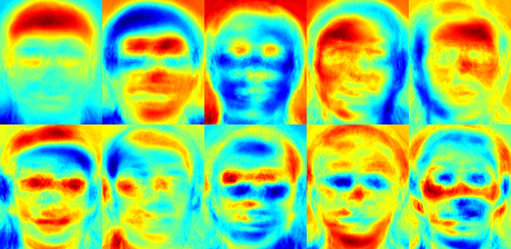
jetカラーマップを使ったので、特定の固有顔の中でグレースケール値がどのように分布しているかを見ることができる。固有顔は顔の特徴を符号化するだけでなく、画像中の照明も符号化していることが分かる(固有顔#4の左からの光、固有顔#5の右からの光を参照):
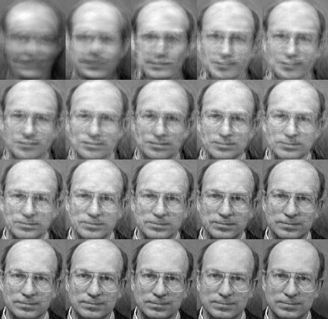
低次元の近似から顔を再構成できることはすでに見た。では、良好な再構成にいくつの固有顔が必要かを見てみよう。\(10,30,\ldots,310\) 個の固有顔でサブプロットを作成する:
10個の固有ベクトルは、良好な画像再構成には明らかに不十分であり、50個の固有ベクトルで重要な顔の特徴を符号化するにはすでに十分かもしれない。AT&T Facedatabase の場合、約300個の固有ベクトルで良好な再構成が得られる。顔認識を成功させるために選ぶべきEigenfacesの数には経験則があるが、それは入力データに大きく依存する。これについて調査を始めるには [329] が最適な出発点である:
固有顔法の中核をなす主成分分析 (PCA) は、データ全体の分散を最大化する特徴の線形結合を見つける。これは明らかにデータを表現する強力な方法だが、クラスをまったく考慮しないため、成分を捨てる際に多くの判別情報が失われる可能性がある。データの分散が外部要因(たとえば光)によって生じている状況を想像してほしい。PCAによって特定される成分には判別情報がまったく含まれているとは限らないため、射影されたサンプルは互いに混ざり合い、分類が不可能になる(例については http://www.bytefish.de/wiki/pca_lda_with_gnu_octave を参照)。
線形判別分析(Linear Discriminant Analysis)は、クラス固有の次元削減を行うもので、偉大な統計学者である Sir R. A. Fisher によって考案された。彼は1936年の論文 The use of multiple measurements in taxonomic problems [96] で、これを花の分類にうまく利用した。クラス間を最もよく分離する特徴の組み合わせを見つけるために、線形判別分析は全体の散らばりを最大化するのではなく、クラス間散布とクラス内散布の比を最大化する。考え方は単純である:同じクラスは互いに密に集まり、異なるクラスは低次元表現において互いにできるだけ遠く離れるべきである。これは Belhumeur、Hespanha、Kriegman にも認識され、彼らは [25] で判別分析を顔認識に適用した。
\(X\) を \(c\) 個のクラスから抽出されたサンプルを持つ確率ベクトルとする:
\[\begin{align*} X & = & \{X_1,X_2,\ldots,X_c\} \\ X_i & = & \{x_1, x_2, \ldots, x_n\} \end{align*}\]
散布行列 \(S_{B}\) と S_{W} は次のように計算される:
\[\begin{align*} S_{B} & = & \sum_{i=1}^{c} N_{i} (\mu_i - \mu)(\mu_i - \mu)^{T} \\ S_{W} & = & \sum_{i=1}^{c} \sum_{x_{j} \in X_{i}} (x_j - \mu_i)(x_j - \mu_i)^{T} \end{align*}\]
ここで \(\mu\) は全体平均である:
\[\mu = \frac{1}{N} \sum_{i=1}^{N} x_i\]
そして \(\mu_i\) はクラス \(i \in \{1,\ldots,c\}\) の平均である:
\[\mu_i = \frac{1}{|X_i|} \sum_{x_j \in X_i} x_j\]
フィッシャーの古典的なアルゴリズムは、クラス分離可能性の基準を最大化する射影 \(W\) を探す:
\[W_{opt} = \operatorname{arg\,max}_{W} \frac{|W^T S_B W|}{|W^T S_W W|}\]
[25] に従うと、この最適化問題の解は一般固有値問題を解くことで得られる:
\[\begin{align*} S_{B} v_{i} & = & \lambda_{i} S_w v_{i} \nonumber \\ S_{W}^{-1} S_{B} v_{i} & = & \lambda_{i} v_{i} \end{align*}\]
解決すべき問題が一つ残っている:\(S_{W}\) のランクは、\(N\) 個のサンプルと \(c\) 個のクラスがある場合、高々 \((N-c)\) である。パターン認識の問題では、サンプル数 \(N\) はほぼ常に入力データの次元(ピクセル数)よりも小さいため、散布行列 \(S_{W}\) は特異(singular)になる([231] を参照)。[25] では、データに対して主成分分析を行い、サンプルを \((N-c)\) 次元空間に射影することでこれを解決した。その後、次元削減されたデータに対して線形判別分析が行われた。なぜなら \(S_{W}\) はもはや特異ではないからである。
すると最適化問題は次のように書き換えられる:
\[\begin{align*} W_{pca} & = & \operatorname{arg\,max}_{W} |W^T S_T W| \\ W_{fld} & = & \operatorname{arg\,max}_{W} \frac{|W^T W_{pca}^T S_{B} W_{pca} W|}{|W^T W_{pca}^T S_{W} W_{pca} W|} \end{align*}\]
サンプルを \((c-1)\) 次元空間へ射影する変換行列 \(W\) は、次のように与えられる:
\[W = W_{fld}^{T} W_{pca}^{T}\]
このデモアプリケーションのソースコードは、このドキュメントに付属するsrcフォルダ内でも入手できる:
この例ではYale顔データベースAを使う。プロットがより見やすいというだけの理由だ。各フィッシャー顔は元の画像と同じ長さを持つため、画像として表示できる。デモは最初の、最大16個のフィッシャー顔を表示(または保存)する:
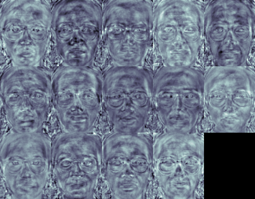
フィッシャー顔法はクラス固有の変換行列を学習するため、固有顔法のように照明を明白に捉えることはない。判別分析は代わりに、人物同士を判別するための顔の特徴を見つける。フィッシャー顔の性能もまた入力データに大きく依存することを述べておくのは重要だ。実際的に言えば、十分に照明された画像だけでフィッシャー顔を学習し、照明の悪いシーンで顔を認識しようとすると、本手法は誤った成分を見つける可能性が高い(そうした特徴は照明の悪い画像では支配的でないかもしれないからだ)。本手法は照明を学習する機会がなかったのだから、これはある意味で論理的である。
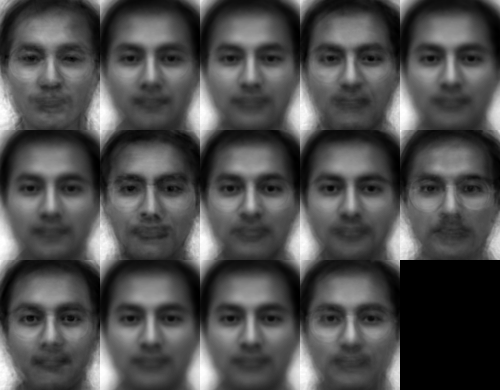
フィッシャー顔は、固有顔と同じように射影された画像の再構成を可能にする。しかし、被験者同士を区別するための特徴だけを特定したので、元の画像の良好な再構成を期待することはできない。フィッシャー顔法では代わりに、サンプル画像を各フィッシャー顔へ射影する。こうすることで、各フィッシャー顔がどの特徴を記述しているかを良好に可視化できる:
違いは人間の目には微妙かもしれないが、いくらかの違いは見て取れるはずだ:
固有顔とフィッシャー顔は、顔認識にやや全体論的なアプローチを取る。データを高次元の画像空間内のどこかにあるベクトルとして扱う。高次元が良くないことは誰もが知っているので、(おそらく)有用な情報が保存される低次元の部分空間が特定される。固有顔のアプローチは全体の散らばりを最大化するが、これは分散が外部要因によって生じる場合に問題を引き起こす可能性がある。なぜなら、すべてのクラスにわたって最大の分散を持つ成分が、必ずしも分類に有用とは限らないからだ(http://www.bytefish.de/wiki/pca_lda_with_gnu_octave を参照)。そこで、いくらかの判別情報を保存するために、線形判別分析を適用し、フィッシャー顔法で説明したとおりに最適化した。フィッシャー顔法はうまく機能した…少なくとも、我々がモデルで仮定した制約のあるシナリオにおいては。
ところが現実は完璧ではない。画像中の完璧な照明設定や、一人につき10枚の異なる画像を保証することは到底できない。では、各人につき画像が1枚しかない場合はどうなるか? 部分空間に対する共分散の推定値はひどく間違っているかもしれず、認識もそうなるだろう。固有顔法がAT&T顔データベースで96%の認識率を持っていたことを覚えているだろうか? このように有用な推定値を得るには、実際に何枚の画像が必要なのか? 以下は、かなり容易な画像データベースであるAT&T顔データベースにおける固有顔法とフィッシャー顔法のRank-1認識率である:
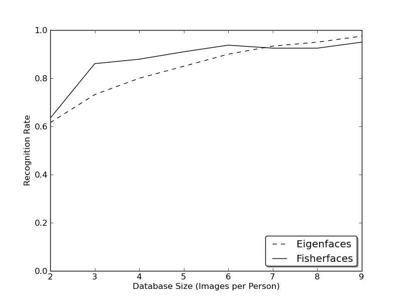
したがって良好な認識率を得るには、各人物について少なくとも8(±1)枚の画像が必要であり、Fisherfaces法はここではあまり役に立たない。上記の実験は、https://github.com/bytefish/facerec にあるfacerecフレームワークで実施した10分割交差検証の結果である。これは出版物ではないため、これらの数値を深い数学的分析で裏付けることはしない。小さな訓練データセットに関する両手法の詳細な分析については、[190] を参照してほしい。
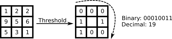
そこで一部の研究は、画像から局所特徴を抽出することに注力した。考え方は、画像全体を高次元ベクトルとして見るのではなく、物体の局所特徴だけを記述するというものだ。このようにして抽出する特徴は、暗黙的に低次元を持つ。素晴らしい考えだ! しかし、与えられた画像表現が照明の変動だけに悩まされるわけではないことにすぐ気づくだろう。画像中のスケール、平行移動、回転といったものを考えてほしい。局所記述は、それらに対して少なくとも多少は頑健でなければならない。SIFTと同様に、局所バイナリパターンの手法は2Dテクスチャ解析にその起源を持つ。局所バイナリパターンの基本的な考え方は、各ピクセルをその近傍と比較することで画像中の局所構造を要約することだ。あるピクセルを中心とし、その近傍と閾値処理する。中心ピクセルの強度が近傍以上であれば1で表し、そうでなければ0とする。各ピクセルについて、次のような2進数が得られる
LBP演算子のより形式的な記述は次のように与えられる:
\[LBP(x_c, y_c) = \sum_{p=0}^{P-1} 2^p s(i_p - i_c)\]
ここで \((x_c, y_c)\) は強度 \(i_c\) を持つ中心ピクセルであり、\(i_n\) は近傍ピクセルの強度である。\(s\) は次のように定義される符号関数である:
\[\begin{equation} s(x) = \begin{cases} 1 & \text{if \(x \geq 0\)}\\ 0 & \text{else} \end{cases} \end{equation}\]
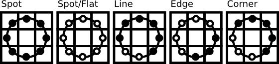
この記述により、画像中の非常にきめ細かい詳細を捉えることができる。実際、著者らはテクスチャ分類において最先端の結果に匹敵することができた。演算子が公開されて間もなく、固定の近傍ではスケールの異なる詳細を符号化できないことが指摘された。そこで演算子は、[4] で可変近傍を使うように拡張された。考え方は、可変半径の円上に任意の数の近傍を配置することであり、これにより次のような近傍を捉えられるようになる:
与えられた点 \((x_c,y_c)\) に対して、近傍 \((x_p,y_p), p \in P\) の位置は次のように計算できる:
\[\begin{align*} x_{p} & = & x_c + R \cos({\frac{2\pi p}{P}})\\ y_{p} & = & y_c - R \sin({\frac{2\pi p}{P}}) \end{align*}\]
ここで \(R\) は円の半径、\(P\) はサンプル点の数である。
この演算子は元のLBPコードの拡張であるため、拡張LBP (Extended LBP)(円形LBP (Circular LBP) とも呼ばれる)と呼ばれることがある。円上の点の座標が画像座標に対応しない場合、その点は補間される。コンピュータサイエンスには巧妙な補間方式が数多くあるが、OpenCVの実装は双線形補間を行う:
\[\begin{align*} f(x,y) \approx \begin{bmatrix} 1-x & x \end{bmatrix} \begin{bmatrix} f(0,0) & f(0,1) \\ f(1,0) & f(1,1) \end{bmatrix} \begin{bmatrix} 1-y \\ y \end{bmatrix}. \end{align*}\]
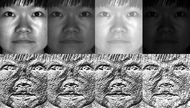
定義により、LBP演算子は単調なグレースケール変換に対して頑健である。人工的に修正した画像のLBP画像を見ることで、これを簡単に確認できる(LBP画像がどのようなものかが分かる!):
そこで残された課題は、空間情報を顔認識モデルにどう組み込むかである。Ahonenらが [4] で提案した表現は、LBP画像を \(m\) 個の局所領域に分割し、それぞれからヒストグラムを抽出するというものだ。空間的に拡張された特徴ベクトルは、局所ヒストグラムを連結する(マージするのではない)ことで得られる。これらのヒストグラムは 局所バイナリパターンヒストグラム (Local Binary Patterns Histograms) と呼ばれる。
このデモアプリケーションのソースコードは、このドキュメントに付属するsrcフォルダ内でも入手できる:
実際のアプリケーションで新しいFaceRecognizerを使う方法を学んだ。このドキュメントを読んだことで、アルゴリズムがどのように動作するかも分かったので、今度は利用可能なアルゴリズムを使って実験する番だ。それらを使い、改良し、OpenCVコミュニティに参加させてほしい!
このドキュメントは、AT&T Database of Faces および Yale Facedatabase A/B の顔画像を使用する親切な許可なしには実現できなかった。
重要: これらの画像を使用する際は、"AT&T Laboratories, Cambridge." のクレジットを明記してほしい。
Database of Faces(旧称 The ORL Database of Faces)は、1992年4月から1994年4月の間に撮影された顔画像の集合を含む。このデータベースは、ケンブリッジ大学工学部のSpeech, Vision and Robotics Groupとの共同で実施された顔認識プロジェクトの文脈で使用された。
40人の異なる被験者それぞれについて、10枚の異なる画像がある。一部の被験者については、照明、表情(目を開ける/閉じる、笑顔/無表情)、顔の細部(眼鏡あり/なし)を変えて、異なる時点で画像が撮影された。すべての画像は、被験者が直立した正面向きの姿勢(多少の横移動は許容)で、暗く均一な背景に対して撮影された。
ファイルはPGM形式である。各画像のサイズは92x112ピクセルで、ピクセルあたり256階調のグレーレベルを持つ。画像は40個のディレクトリ(被験者ごとに1つ)に整理されており、それぞれ sX という形式の名前を持つ(Xは1から40までの被験者番号を示す)。これらの各ディレクトリには、その被験者の10枚の異なる画像があり、Y.pgm という形式の名前を持つ(Yはその被験者に対する1から10までの画像番号)。
データベースのコピーは次から取得できる: http://www.cl.cam.ac.uk/research/dtg/attarchive/pub/data/att_faces.zip。
著者の許可を得て、少数の画像(たとえば被験者1とそのすべてのバリエーション)と、Yale Facedatabase AまたはYale Facedatabase Bのいずれかから得られたフィッシャー顔や固有顔などのすべての画像を表示することが許可されている。
Yale Face Database A(サイズ6.4MB)は、15人の個人のGIF形式のグレースケール画像165枚を含む。被験者ごとに11枚の画像があり、異なる表情または構成ごとに1枚ずつである: center-light、w/glasses、happy、left-light、w/no glasses、normal、right-light、sad、sleepy、surprised、wink。(出典: http://cvc.yale.edu/projects/yalefaces/yalefaces.html)
著者の許可を得て、少数の画像(たとえば被験者1とそのすべてのバリエーション)と、Yale Facedatabase AまたはYale Facedatabase Bのいずれかから得られたフィッシャー顔や固有顔などのすべての画像を表示することが許可されている。
拡張Yale Face Database Bは、9種類のポーズと64種類の照明条件のもとでの28人の被験者の画像16128枚を含む。このデータベースのデータ形式はYale Face Database Bと同じである。データ形式の詳細については、Yale Face Database Bのホームページ(またはこのページのコピー)を参照してほしい。
拡張Yale Face Database Bは研究目的で自由に使用できる。このデータベースを使用するすべての出版物では、"the Exteded Yale Face Database B" の使用を明記し、Athinodoros Georghiades、Peter Belhumeur、David Kriegmanの論文 "From Few to Many: Illumination Cone Models for Face Recognition under Variable Lighting and Pose"(PAMI, 2001, [bibtex])を参照すべきである。
10人の被験者を含む元のYale Face Database Bに対する拡張データベースは、Kuang-Chih Lee、Jeffrey Ho、David Kriegmanにより "Acquiring Linear Subspaces for Face Recognition under Variable Lighting, PAMI, May, 2005 <a href="http://vision.ucsd.edu/~leekc/papers/9pltsIEEE.pdf" target="_blank" >[pdf]</a>." で初めて報告された。実験で使用したすべてのテスト画像データは、手作業で位置合わせ、切り出しが行われ、その後168x192の画像にリサイズされている。切り出した画像を用いた実験結果を発表する場合は、PAMI2005の論文も参照してほしい。(出典: http://vision.ucsd.edu/~leekc/ExtYaleDatabase/ExtYaleB.html)
CSVファイルを手作業で作成したくはないはずだ。CSVファイルを自動的に作成してくれる小さなPythonスクリプト create_csv.py(このチュートリアルに付属する src/create_csv.py にある)を用意しておいた。画像を次のような階層(/basepath/<subject>/<image.ext>)で持っている場合:
そのうえで、次のように単純に create_csv.py at を呼び出せばよい。ここで 'at' はフォルダへのbasepathであり、出力を保存できる:
見つけられない場合のために、スクリプトを以下に示す:
#!/usr/bin/env python

import sys
import os.path

# This is a tiny script to help you creating a CSV file from a face
# database with a similar hierarchie:
#
#  philipp@mango:~/facerec/data/at$ tree
#  .
#  |-- README
#  |-- s1
#  |   |-- 1.pgm
#  |   |-- ...
#  |   |-- 10.pgm
#  |-- s2
#  |   |-- 1.pgm
#  |   |-- ...
#  |   |-- 10.pgm
#  ...
#  |-- s40
#  |   |-- 1.pgm
#  |   |-- ...
#  |   |-- 10.pgm
#

if __name__ == "__main__":

    if len(sys.argv) != 2:
        print "usage: create_csv <base_path>"
        sys.exit(1)

    BASE_PATH=sys.argv[1]
    SEPARATOR=";"

    label = 0
    for dirname, dirnames, filenames in os.walk(BASE_PATH):
        for subdirname in dirnames:
            subject_path = os.path.join(dirname, subdirname)
            for filename in os.listdir(subject_path):
                abs_path = "%s/%s" % (subject_path, filename)
                print "%s%s%d" % (abs_path, SEPARATOR, label)
            label = label + 1
画像データの正確な位置合わせは、できるだけ多くの詳細が必要となる感情検出のようなタスクでは特に重要である。信じてほしい…これを手作業でやりたくはないはずだ。そこで小さなPythonスクリプトを用意しておいた。このコードは本当に使いやすい。顔画像をスケーリング、回転、切り出しするには、CropFace(image, eye_left, eye_right, offset_pct, dest_sz) を呼び出すだけでよい。ここで:
すべての画像に同じ offset_pct と dest_sz を使えば、それらはすべて目の位置で位置合わせされる。
#!/usr/bin/env python
# Software License Agreement (BSD License)
#
# Copyright (c) 2012, Philipp Wagner
# All rights reserved.
#
# Redistribution and use in source and binary forms, with or without
# modification, are permitted provided that the following conditions
# are met:
#
#  * Redistributions of source code must retain the above copyright
#    notice, this list of conditions and the following disclaimer.
#  * Redistributions in binary form must reproduce the above
#    copyright notice, this list of conditions and the following
#    disclaimer in the documentation and/or other materials provided
#    with the distribution.
#  * Neither the name of the author nor the names of its
#    contributors may be used to endorse or promote products derived
#    from this software without specific prior written permission.
#
# THIS SOFTWARE IS PROVIDED BY THE COPYRIGHT HOLDERS AND CONTRIBUTORS
# "AS IS" AND ANY EXPRESS OR IMPLIED WARRANTIES, INCLUDING, BUT NOT
# LIMITED TO, THE IMPLIED WARRANTIES OF MERCHANTABILITY AND FITNESS
# FOR A PARTICULAR PURPOSE ARE DISCLAIMED. IN NO EVENT SHALL THE
# COPYRIGHT OWNER OR CONTRIBUTORS BE LIABLE FOR ANY DIRECT, INDIRECT,
# INCIDENTAL, SPECIAL, EXEMPLARY, OR CONSEQUENTIAL DAMAGES (INCLUDING,
# BUT NOT LIMITED TO, PROCUREMENT OF SUBSTITUTE GOODS OR SERVICES;
# LOSS OF USE, DATA, OR PROFITS; OR BUSINESS INTERRUPTION) HOWEVER
# CAUSED AND ON ANY THEORY OF LIABILITY, WHETHER IN CONTRACT, STRICT
# LIABILITY, OR TORT (INCLUDING NEGLIGENCE OR OTHERWISE) ARISING IN
# ANY WAY OUT OF THE USE OF THIS SOFTWARE, EVEN IF ADVISED OF THE
# POSSIBILITY OF SUCH DAMAGE.

import sys, math, Image

def Distance(p1,p2):
  dx = p2[0] - p1[0]
  dy = p2[1] - p1[1]
  return math.sqrt(dx*dx+dy*dy)

def ScaleRotateTranslate(image, angle, center = None, new_center = None, scale = None, resample=Image.BICUBIC):
  if (scale is None) and (center is None):
    return image.rotate(angle=angle, resample=resample)
  nx,ny = x,y = center
  sx=sy=1.0
  if new_center:
    (nx,ny) = new_center
  if scale:
    (sx,sy) = (scale, scale)
  cosine = math.cos(angle)
  sine = math.sin(angle)
  a = cosine/sx
  b = sine/sx
  c = x-nx*a-ny*b
  d = -sine/sy
  e = cosine/sy
  f = y-nx*d-ny*e
  return image.transform(image.size, Image.AFFINE, (a,b,c,d,e,f), resample=resample)

def CropFace(image, eye_left=(0,0), eye_right=(0,0), offset_pct=(0.2,0.2), dest_sz = (70,70)):
  # calculate offsets in original image
  offset_h = math.floor(float(offset_pct[0])*dest_sz[0])
  offset_v = math.floor(float(offset_pct[1])*dest_sz[1])
  # get the direction
  eye_direction = (eye_right[0] - eye_left[0], eye_right[1] - eye_left[1])
  # calc rotation angle in radians
  rotation = -math.atan2(float(eye_direction[1]),float(eye_direction[0]))
  # distance between them
  dist = Distance(eye_left, eye_right)
  # calculate the reference eye-width
  reference = dest_sz[0] - 2.0*offset_h
  # scale factor
  scale = float(dist)/float(reference)
  # rotate original around the left eye
  image = ScaleRotateTranslate(image, center=eye_left, angle=rotation)
  # crop the rotated image
  crop_xy = (eye_left[0] - scale*offset_h, eye_left[1] - scale*offset_v)
  crop_size = (dest_sz[0]*scale, dest_sz[1]*scale)
  image = image.crop((int(crop_xy[0]), int(crop_xy[1]), int(crop_xy[0]+crop_size[0]), int(crop_xy[1]+crop_size[1])))
  # resize it
  image = image.resize(dest_sz, Image.ANTIALIAS)
  return image

def readFileNames():
    try:
        inFile = open('path_to_created_csv_file.csv')
    except:
        raise IOError('There is no file named path_to_created_csv_file.csv in current directory.')
        return False

    picPath = []
    picIndex = []

    for line in inFile.readlines():
        if line != '':
            fields = line.rstrip().split(';')
            picPath.append(fields[0])
            picIndex.append(int(fields[1]))

    return (picPath, picIndex)


if __name__ == "__main__":
  [images, indexes]=readFileNames()
if not os.path.exists("modified"):
    os.makedirs("modified")
for img in images:
    image =  Image.open(img)
    CropFace(image, eye_left=(252,364), eye_right=(420,366), offset_pct=(0.1,0.1), dest_sz=(200,200)).save("modified/"+img.rstrip().split('/')[1]+"_10_10_200_200.jpg")
    CropFace(image, eye_left=(252,364), eye_right=(420,366), offset_pct=(0.2,0.2), dest_sz=(200,200)).save("modified/"+img.rstrip().split('/')[1]+"_20_20_200_200.jpg")
    CropFace(image, eye_left=(252,364), eye_right=(420,366), offset_pct=(0.3,0.3), dest_sz=(200,200)).save("modified/"+img.rstrip().split('/')[1]+"_30_30_200_200.jpg")
    CropFace(image, eye_left=(252,364), eye_right=(420,366), offset_pct=(0.2,0.2)).save("modified/"+img.rstrip().split('/')[1]+"_20_20_70_70.jpg")
パブリックドメインのライセンスであるこのアーノルド・シュワルツェネッガーの写真が与えられたとしよう。目の (x,y) 位置はおおよそ左目が (252,364)、右目が (420,366) である。あとは、スケーリング・回転・切り抜き後の顔が持つべき水平オフセット、垂直オフセット、サイズを定義すればよい。
いくつかの例を示す:
| 設定 | 切り抜き・スケーリング・回転された顔 |
|---|---|
| 0.1 (10%), 0.1 (10%), (200,200) |  |
| 0.2 (20%), 0.2 (20%), (200,200) |  |
| 0.3 (30%), 0.3 (30%), (200,200) |  |
| 0.2 (20%), 0.2 (20%), (70,70) |  |
/home/philipp/facerec/data/at/s13/2.pgm;12
/home/philipp/facerec/data/at/s13/7.pgm;12
/home/philipp/facerec/data/at/s13/6.pgm;12
/home/philipp/facerec/data/at/s13/9.pgm;12
/home/philipp/facerec/data/at/s13/5.pgm;12
/home/philipp/facerec/data/at/s13/3.pgm;12
/home/philipp/facerec/data/at/s13/4.pgm;12
/home/philipp/facerec/data/at/s13/10.pgm;12
/home/philipp/facerec/data/at/s13/8.pgm;12
/home/philipp/facerec/data/at/s13/1.pgm;12
/home/philipp/facerec/data/at/s17/2.pgm;16
/home/philipp/facerec/data/at/s17/7.pgm;16
/home/philipp/facerec/data/at/s17/6.pgm;16
/home/philipp/facerec/data/at/s17/9.pgm;16
/home/philipp/facerec/data/at/s17/5.pgm;16
/home/philipp/facerec/data/at/s17/3.pgm;16
/home/philipp/facerec/data/at/s17/4.pgm;16
/home/philipp/facerec/data/at/s17/10.pgm;16
/home/philipp/facerec/data/at/s17/8.pgm;16
/home/philipp/facerec/data/at/s17/1.pgm;16
/home/philipp/facerec/data/at/s32/2.pgm;31
/home/philipp/facerec/data/at/s32/7.pgm;31
/home/philipp/facerec/data/at/s32/6.pgm;31
/home/philipp/facerec/data/at/s32/9.pgm;31
/home/philipp/facerec/data/at/s32/5.pgm;31
/home/philipp/facerec/data/at/s32/3.pgm;31
/home/philipp/facerec/data/at/s32/4.pgm;31
/home/philipp/facerec/data/at/s32/10.pgm;31
/home/philipp/facerec/data/at/s32/8.pgm;31
/home/philipp/facerec/data/at/s32/1.pgm;31
/home/philipp/facerec/data/at/s10/2.pgm;9
/home/philipp/facerec/data/at/s10/7.pgm;9
/home/philipp/facerec/data/at/s10/6.pgm;9
/home/philipp/facerec/data/at/s10/9.pgm;9
/home/philipp/facerec/data/at/s10/5.pgm;9
/home/philipp/facerec/data/at/s10/3.pgm;9
/home/philipp/facerec/data/at/s10/4.pgm;9
/home/philipp/facerec/data/at/s10/10.pgm;9
/home/philipp/facerec/data/at/s10/8.pgm;9
/home/philipp/facerec/data/at/s10/1.pgm;9
/home/philipp/facerec/data/at/s27/2.pgm;26
/home/philipp/facerec/data/at/s27/7.pgm;26
/home/philipp/facerec/data/at/s27/6.pgm;26
/home/philipp/facerec/data/at/s27/9.pgm;26
/home/philipp/facerec/data/at/s27/5.pgm;26
/home/philipp/facerec/data/at/s27/3.pgm;26
/home/philipp/facerec/data/at/s27/4.pgm;26
/home/philipp/facerec/data/at/s27/10.pgm;26
/home/philipp/facerec/data/at/s27/8.pgm;26
/home/philipp/facerec/data/at/s27/1.pgm;26
/home/philipp/facerec/data/at/s5/2.pgm;4
/home/philipp/facerec/data/at/s5/7.pgm;4
/home/philipp/facerec/data/at/s5/6.pgm;4
/home/philipp/facerec/data/at/s5/9.pgm;4
/home/philipp/facerec/data/at/s5/5.pgm;4
/home/philipp/facerec/data/at/s5/3.pgm;4
/home/philipp/facerec/data/at/s5/4.pgm;4
/home/philipp/facerec/data/at/s5/10.pgm;4
/home/philipp/facerec/data/at/s5/8.pgm;4
/home/philipp/facerec/data/at/s5/1.pgm;4
/home/philipp/facerec/data/at/s20/2.pgm;19
/home/philipp/facerec/data/at/s20/7.pgm;19
/home/philipp/facerec/data/at/s20/6.pgm;19
/home/philipp/facerec/data/at/s20/9.pgm;19
/home/philipp/facerec/data/at/s20/5.pgm;19
/home/philipp/facerec/data/at/s20/3.pgm;19
/home/philipp/facerec/data/at/s20/4.pgm;19
/home/philipp/facerec/data/at/s20/10.pgm;19
/home/philipp/facerec/data/at/s20/8.pgm;19
/home/philipp/facerec/data/at/s20/1.pgm;19
/home/philipp/facerec/data/at/s30/2.pgm;29
/home/philipp/facerec/data/at/s30/7.pgm;29
/home/philipp/facerec/data/at/s30/6.pgm;29
/home/philipp/facerec/data/at/s30/9.pgm;29
/home/philipp/facerec/data/at/s30/5.pgm;29
/home/philipp/facerec/data/at/s30/3.pgm;29
/home/philipp/facerec/data/at/s30/4.pgm;29
/home/philipp/facerec/data/at/s30/10.pgm;29
/home/philipp/facerec/data/at/s30/8.pgm;29
/home/philipp/facerec/data/at/s30/1.pgm;29
/home/philipp/facerec/data/at/s39/2.pgm;38
/home/philipp/facerec/data/at/s39/7.pgm;38
/home/philipp/facerec/data/at/s39/6.pgm;38
/home/philipp/facerec/data/at/s39/9.pgm;38
/home/philipp/facerec/data/at/s39/5.pgm;38
/home/philipp/facerec/data/at/s39/3.pgm;38
/home/philipp/facerec/data/at/s39/4.pgm;38
/home/philipp/facerec/data/at/s39/10.pgm;38
/home/philipp/facerec/data/at/s39/8.pgm;38
/home/philipp/facerec/data/at/s39/1.pgm;38
/home/philipp/facerec/data/at/s35/2.pgm;34
/home/philipp/facerec/data/at/s35/7.pgm;34
/home/philipp/facerec/data/at/s35/6.pgm;34
/home/philipp/facerec/data/at/s35/9.pgm;34
/home/philipp/facerec/data/at/s35/5.pgm;34
/home/philipp/facerec/data/at/s35/3.pgm;34
/home/philipp/facerec/data/at/s35/4.pgm;34
/home/philipp/facerec/data/at/s35/10.pgm;34
/home/philipp/facerec/data/at/s35/8.pgm;34
/home/philipp/facerec/data/at/s35/1.pgm;34
/home/philipp/facerec/data/at/s23/2.pgm;22
/home/philipp/facerec/data/at/s23/7.pgm;22
/home/philipp/facerec/data/at/s23/6.pgm;22
/home/philipp/facerec/data/at/s23/9.pgm;22
/home/philipp/facerec/data/at/s23/5.pgm;22
/home/philipp/facerec/data/at/s23/3.pgm;22
/home/philipp/facerec/data/at/s23/4.pgm;22
/home/philipp/facerec/data/at/s23/10.pgm;22
/home/philipp/facerec/data/at/s23/8.pgm;22
/home/philipp/facerec/data/at/s23/1.pgm;22
/home/philipp/facerec/data/at/s4/2.pgm;3
/home/philipp/facerec/data/at/s4/7.pgm;3
/home/philipp/facerec/data/at/s4/6.pgm;3
/home/philipp/facerec/data/at/s4/9.pgm;3
/home/philipp/facerec/data/at/s4/5.pgm;3
/home/philipp/facerec/data/at/s4/3.pgm;3
/home/philipp/facerec/data/at/s4/4.pgm;3
/home/philipp/facerec/data/at/s4/10.pgm;3
/home/philipp/facerec/data/at/s4/8.pgm;3
/home/philipp/facerec/data/at/s4/1.pgm;3
/home/philipp/facerec/data/at/s9/2.pgm;8
/home/philipp/facerec/data/at/s9/7.pgm;8
/home/philipp/facerec/data/at/s9/6.pgm;8
/home/philipp/facerec/data/at/s9/9.pgm;8
/home/philipp/facerec/data/at/s9/5.pgm;8
/home/philipp/facerec/data/at/s9/3.pgm;8
/home/philipp/facerec/data/at/s9/4.pgm;8
/home/philipp/facerec/data/at/s9/10.pgm;8
/home/philipp/facerec/data/at/s9/8.pgm;8
/home/philipp/facerec/data/at/s9/1.pgm;8
/home/philipp/facerec/data/at/s37/2.pgm;36
/home/philipp/facerec/data/at/s37/7.pgm;36
/home/philipp/facerec/data/at/s37/6.pgm;36
/home/philipp/facerec/data/at/s37/9.pgm;36
/home/philipp/facerec/data/at/s37/5.pgm;36
/home/philipp/facerec/data/at/s37/3.pgm;36
/home/philipp/facerec/data/at/s37/4.pgm;36
/home/philipp/facerec/data/at/s37/10.pgm;36
/home/philipp/facerec/data/at/s37/8.pgm;36
/home/philipp/facerec/data/at/s37/1.pgm;36
/home/philipp/facerec/data/at/s24/2.pgm;23
/home/philipp/facerec/data/at/s24/7.pgm;23
/home/philipp/facerec/data/at/s24/6.pgm;23
/home/philipp/facerec/data/at/s24/9.pgm;23
/home/philipp/facerec/data/at/s24/5.pgm;23
/home/philipp/facerec/data/at/s24/3.pgm;23
/home/philipp/facerec/data/at/s24/4.pgm;23
/home/philipp/facerec/data/at/s24/10.pgm;23
/home/philipp/facerec/data/at/s24/8.pgm;23
/home/philipp/facerec/data/at/s24/1.pgm;23
/home/philipp/facerec/data/at/s19/2.pgm;18
/home/philipp/facerec/data/at/s19/7.pgm;18
/home/philipp/facerec/data/at/s19/6.pgm;18
/home/philipp/facerec/data/at/s19/9.pgm;18
/home/philipp/facerec/data/at/s19/5.pgm;18
/home/philipp/facerec/data/at/s19/3.pgm;18
/home/philipp/facerec/data/at/s19/4.pgm;18
/home/philipp/facerec/data/at/s19/10.pgm;18
/home/philipp/facerec/data/at/s19/8.pgm;18
/home/philipp/facerec/data/at/s19/1.pgm;18
/home/philipp/facerec/data/at/s8/2.pgm;7
/home/philipp/facerec/data/at/s8/7.pgm;7
/home/philipp/facerec/data/at/s8/6.pgm;7
/home/philipp/facerec/data/at/s8/9.pgm;7
/home/philipp/facerec/data/at/s8/5.pgm;7
/home/philipp/facerec/data/at/s8/3.pgm;7
/home/philipp/facerec/data/at/s8/4.pgm;7
/home/philipp/facerec/data/at/s8/10.pgm;7
/home/philipp/facerec/data/at/s8/8.pgm;7
/home/philipp/facerec/data/at/s8/1.pgm;7
/home/philipp/facerec/data/at/s21/2.pgm;20
/home/philipp/facerec/data/at/s21/7.pgm;20
/home/philipp/facerec/data/at/s21/6.pgm;20
/home/philipp/facerec/data/at/s21/9.pgm;20
/home/philipp/facerec/data/at/s21/5.pgm;20
/home/philipp/facerec/data/at/s21/3.pgm;20
/home/philipp/facerec/data/at/s21/4.pgm;20
/home/philipp/facerec/data/at/s21/10.pgm;20
/home/philipp/facerec/data/at/s21/8.pgm;20
/home/philipp/facerec/data/at/s21/1.pgm;20
/home/philipp/facerec/data/at/s1/2.pgm;0
/home/philipp/facerec/data/at/s1/7.pgm;0
/home/philipp/facerec/data/at/s1/6.pgm;0
/home/philipp/facerec/data/at/s1/9.pgm;0
/home/philipp/facerec/data/at/s1/5.pgm;0
/home/philipp/facerec/data/at/s1/3.pgm;0
/home/philipp/facerec/data/at/s1/4.pgm;0
/home/philipp/facerec/data/at/s1/10.pgm;0
/home/philipp/facerec/data/at/s1/8.pgm;0
/home/philipp/facerec/data/at/s1/1.pgm;0
/home/philipp/facerec/data/at/s7/2.pgm;6
/home/philipp/facerec/data/at/s7/7.pgm;6
/home/philipp/facerec/data/at/s7/6.pgm;6
/home/philipp/facerec/data/at/s7/9.pgm;6
/home/philipp/facerec/data/at/s7/5.pgm;6
/home/philipp/facerec/data/at/s7/3.pgm;6
/home/philipp/facerec/data/at/s7/4.pgm;6
/home/philipp/facerec/data/at/s7/10.pgm;6
/home/philipp/facerec/data/at/s7/8.pgm;6
/home/philipp/facerec/data/at/s7/1.pgm;6
/home/philipp/facerec/data/at/s16/2.pgm;15
/home/philipp/facerec/data/at/s16/7.pgm;15
/home/philipp/facerec/data/at/s16/6.pgm;15
/home/philipp/facerec/data/at/s16/9.pgm;15
/home/philipp/facerec/data/at/s16/5.pgm;15
/home/philipp/facerec/data/at/s16/3.pgm;15
/home/philipp/facerec/data/at/s16/4.pgm;15
/home/philipp/facerec/data/at/s16/10.pgm;15
/home/philipp/facerec/data/at/s16/8.pgm;15
/home/philipp/facerec/data/at/s16/1.pgm;15
/home/philipp/facerec/data/at/s36/2.pgm;35
/home/philipp/facerec/data/at/s36/7.pgm;35
/home/philipp/facerec/data/at/s36/6.pgm;35
/home/philipp/facerec/data/at/s36/9.pgm;35
/home/philipp/facerec/data/at/s36/5.pgm;35
/home/philipp/facerec/data/at/s36/3.pgm;35
/home/philipp/facerec/data/at/s36/4.pgm;35
/home/philipp/facerec/data/at/s36/10.pgm;35
/home/philipp/facerec/data/at/s36/8.pgm;35
/home/philipp/facerec/data/at/s36/1.pgm;35
/home/philipp/facerec/data/at/s25/2.pgm;24
/home/philipp/facerec/data/at/s25/7.pgm;24
/home/philipp/facerec/data/at/s25/6.pgm;24
/home/philipp/facerec/data/at/s25/9.pgm;24
/home/philipp/facerec/data/at/s25/5.pgm;24
/home/philipp/facerec/data/at/s25/3.pgm;24
/home/philipp/facerec/data/at/s25/4.pgm;24
/home/philipp/facerec/data/at/s25/10.pgm;24
/home/philipp/facerec/data/at/s25/8.pgm;24
/home/philipp/facerec/data/at/s25/1.pgm;24
/home/philipp/facerec/data/at/s14/2.pgm;13
/home/philipp/facerec/data/at/s14/7.pgm;13
/home/philipp/facerec/data/at/s14/6.pgm;13
/home/philipp/facerec/data/at/s14/9.pgm;13
/home/philipp/facerec/data/at/s14/5.pgm;13
/home/philipp/facerec/data/at/s14/3.pgm;13
/home/philipp/facerec/data/at/s14/4.pgm;13
/home/philipp/facerec/data/at/s14/10.pgm;13
/home/philipp/facerec/data/at/s14/8.pgm;13
/home/philipp/facerec/data/at/s14/1.pgm;13
/home/philipp/facerec/data/at/s34/2.pgm;33
/home/philipp/facerec/data/at/s34/7.pgm;33
/home/philipp/facerec/data/at/s34/6.pgm;33
/home/philipp/facerec/data/at/s34/9.pgm;33
/home/philipp/facerec/data/at/s34/5.pgm;33
/home/philipp/facerec/data/at/s34/3.pgm;33
/home/philipp/facerec/data/at/s34/4.pgm;33
/home/philipp/facerec/data/at/s34/10.pgm;33
/home/philipp/facerec/data/at/s34/8.pgm;33
/home/philipp/facerec/data/at/s34/1.pgm;33
/home/philipp/facerec/data/at/s11/2.pgm;10
/home/philipp/facerec/data/at/s11/7.pgm;10
/home/philipp/facerec/data/at/s11/6.pgm;10
/home/philipp/facerec/data/at/s11/9.pgm;10
/home/philipp/facerec/data/at/s11/5.pgm;10
/home/philipp/facerec/data/at/s11/3.pgm;10
/home/philipp/facerec/data/at/s11/4.pgm;10
/home/philipp/facerec/data/at/s11/10.pgm;10
/home/philipp/facerec/data/at/s11/8.pgm;10
/home/philipp/facerec/data/at/s11/1.pgm;10
/home/philipp/facerec/data/at/s26/2.pgm;25
/home/philipp/facerec/data/at/s26/7.pgm;25
/home/philipp/facerec/data/at/s26/6.pgm;25
/home/philipp/facerec/data/at/s26/9.pgm;25
/home/philipp/facerec/data/at/s26/5.pgm;25
/home/philipp/facerec/data/at/s26/3.pgm;25
/home/philipp/facerec/data/at/s26/4.pgm;25
/home/philipp/facerec/data/at/s26/10.pgm;25
/home/philipp/facerec/data/at/s26/8.pgm;25
/home/philipp/facerec/data/at/s26/1.pgm;25
/home/philipp/facerec/data/at/s18/2.pgm;17
/home/philipp/facerec/data/at/s18/7.pgm;17
/home/philipp/facerec/data/at/s18/6.pgm;17
/home/philipp/facerec/data/at/s18/9.pgm;17
/home/philipp/facerec/data/at/s18/5.pgm;17
/home/philipp/facerec/data/at/s18/3.pgm;17
/home/philipp/facerec/data/at/s18/4.pgm;17
/home/philipp/facerec/data/at/s18/10.pgm;17
/home/philipp/facerec/data/at/s18/8.pgm;17
/home/philipp/facerec/data/at/s18/1.pgm;17
/home/philipp/facerec/data/at/s29/2.pgm;28
/home/philipp/facerec/data/at/s29/7.pgm;28
/home/philipp/facerec/data/at/s29/6.pgm;28
/home/philipp/facerec/data/at/s29/9.pgm;28
/home/philipp/facerec/data/at/s29/5.pgm;28
/home/philipp/facerec/data/at/s29/3.pgm;28
/home/philipp/facerec/data/at/s29/4.pgm;28
/home/philipp/facerec/data/at/s29/10.pgm;28
/home/philipp/facerec/data/at/s29/8.pgm;28
/home/philipp/facerec/data/at/s29/1.pgm;28
/home/philipp/facerec/data/at/s33/2.pgm;32
/home/philipp/facerec/data/at/s33/7.pgm;32
/home/philipp/facerec/data/at/s33/6.pgm;32
/home/philipp/facerec/data/at/s33/9.pgm;32
/home/philipp/facerec/data/at/s33/5.pgm;32
/home/philipp/facerec/data/at/s33/3.pgm;32
/home/philipp/facerec/data/at/s33/4.pgm;32
/home/philipp/facerec/data/at/s33/10.pgm;32
/home/philipp/facerec/data/at/s33/8.pgm;32
/home/philipp/facerec/data/at/s33/1.pgm;32
/home/philipp/facerec/data/at/s12/2.pgm;11
/home/philipp/facerec/data/at/s12/7.pgm;11
/home/philipp/facerec/data/at/s12/6.pgm;11
/home/philipp/facerec/data/at/s12/9.pgm;11
/home/philipp/facerec/data/at/s12/5.pgm;11
/home/philipp/facerec/data/at/s12/3.pgm;11
/home/philipp/facerec/data/at/s12/4.pgm;11
/home/philipp/facerec/data/at/s12/10.pgm;11
/home/philipp/facerec/data/at/s12/8.pgm;11
/home/philipp/facerec/data/at/s12/1.pgm;11
/home/philipp/facerec/data/at/s6/2.pgm;5
/home/philipp/facerec/data/at/s6/7.pgm;5
/home/philipp/facerec/data/at/s6/6.pgm;5
/home/philipp/facerec/data/at/s6/9.pgm;5
/home/philipp/facerec/data/at/s6/5.pgm;5
/home/philipp/facerec/data/at/s6/3.pgm;5
/home/philipp/facerec/data/at/s6/4.pgm;5
/home/philipp/facerec/data/at/s6/10.pgm;5
/home/philipp/facerec/data/at/s6/8.pgm;5
/home/philipp/facerec/data/at/s6/1.pgm;5
/home/philipp/facerec/data/at/s22/2.pgm;21
/home/philipp/facerec/data/at/s22/7.pgm;21
/home/philipp/facerec/data/at/s22/6.pgm;21
/home/philipp/facerec/data/at/s22/9.pgm;21
/home/philipp/facerec/data/at/s22/5.pgm;21
/home/philipp/facerec/data/at/s22/3.pgm;21
/home/philipp/facerec/data/at/s22/4.pgm;21
/home/philipp/facerec/data/at/s22/10.pgm;21
/home/philipp/facerec/data/at/s22/8.pgm;21
/home/philipp/facerec/data/at/s22/1.pgm;21
/home/philipp/facerec/data/at/s15/2.pgm;14
/home/philipp/facerec/data/at/s15/7.pgm;14
/home/philipp/facerec/data/at/s15/6.pgm;14
/home/philipp/facerec/data/at/s15/9.pgm;14
/home/philipp/facerec/data/at/s15/5.pgm;14
/home/philipp/facerec/data/at/s15/3.pgm;14
/home/philipp/facerec/data/at/s15/4.pgm;14
/home/philipp/facerec/data/at/s15/10.pgm;14
/home/philipp/facerec/data/at/s15/8.pgm;14
/home/philipp/facerec/data/at/s15/1.pgm;14
/home/philipp/facerec/data/at/s2/2.pgm;1
/home/philipp/facerec/data/at/s2/7.pgm;1
/home/philipp/facerec/data/at/s2/6.pgm;1
/home/philipp/facerec/data/at/s2/9.pgm;1
/home/philipp/facerec/data/at/s2/5.pgm;1
/home/philipp/facerec/data/at/s2/3.pgm;1
/home/philipp/facerec/data/at/s2/4.pgm;1
/home/philipp/facerec/data/at/s2/10.pgm;1
/home/philipp/facerec/data/at/s2/8.pgm;1
/home/philipp/facerec/data/at/s2/1.pgm;1
/home/philipp/facerec/data/at/s31/2.pgm;30
/home/philipp/facerec/data/at/s31/7.pgm;30
/home/philipp/facerec/data/at/s31/6.pgm;30
/home/philipp/facerec/data/at/s31/9.pgm;30
/home/philipp/facerec/data/at/s31/5.pgm;30
/home/philipp/facerec/data/at/s31/3.pgm;30
/home/philipp/facerec/data/at/s31/4.pgm;30
/home/philipp/facerec/data/at/s31/10.pgm;30
/home/philipp/facerec/data/at/s31/8.pgm;30
/home/philipp/facerec/data/at/s31/1.pgm;30
/home/philipp/facerec/data/at/s28/2.pgm;27
/home/philipp/facerec/data/at/s28/7.pgm;27
/home/philipp/facerec/data/at/s28/6.pgm;27
/home/philipp/facerec/data/at/s28/9.pgm;27
/home/philipp/facerec/data/at/s28/5.pgm;27
/home/philipp/facerec/data/at/s28/3.pgm;27
/home/philipp/facerec/data/at/s28/4.pgm;27
/home/philipp/facerec/data/at/s28/10.pgm;27
/home/philipp/facerec/data/at/s28/8.pgm;27
/home/philipp/facerec/data/at/s28/1.pgm;27
/home/philipp/facerec/data/at/s40/2.pgm;39
/home/philipp/facerec/data/at/s40/7.pgm;39
/home/philipp/facerec/data/at/s40/6.pgm;39
/home/philipp/facerec/data/at/s40/9.pgm;39
/home/philipp/facerec/data/at/s40/5.pgm;39
/home/philipp/facerec/data/at/s40/3.pgm;39
/home/philipp/facerec/data/at/s40/4.pgm;39
/home/philipp/facerec/data/at/s40/10.pgm;39
/home/philipp/facerec/data/at/s40/8.pgm;39
/home/philipp/facerec/data/at/s40/1.pgm;39
/home/philipp/facerec/data/at/s3/2.pgm;2
/home/philipp/facerec/data/at/s3/7.pgm;2
/home/philipp/facerec/data/at/s3/6.pgm;2
/home/philipp/facerec/data/at/s3/9.pgm;2
/home/philipp/facerec/data/at/s3/5.pgm;2
/home/philipp/facerec/data/at/s3/3.pgm;2
/home/philipp/facerec/data/at/s3/4.pgm;2
/home/philipp/facerec/data/at/s3/10.pgm;2
/home/philipp/facerec/data/at/s3/8.pgm;2
/home/philipp/facerec/data/at/s3/1.pgm;2
/home/philipp/facerec/data/at/s38/2.pgm;37
/home/philipp/facerec/data/at/s38/7.pgm;37
/home/philipp/facerec/data/at/s38/6.pgm;37
/home/philipp/facerec/data/at/s38/9.pgm;37
/home/philipp/facerec/data/at/s38/5.pgm;37
/home/philipp/facerec/data/at/s38/3.pgm;37
/home/philipp/facerec/data/at/s38/4.pgm;37
/home/philipp/facerec/data/at/s38/10.pgm;37
/home/philipp/facerec/data/at/s38/8.pgm;37
/home/philipp/facerec/data/at/s38/1.pgm;37